Chapter 16 RCT analysis and prediction in bmbstats
In this chapter I will demonstrate how to analyze simple randomized controlled trials (RCTs) from both explanatory and predictive perspectives using bmbstats package and functions. As a refresher, please consider re-reading Causal inference chapter.
16.1 Data Generating Process behind RCT
The following image is re-posted from the Causal inference chapter, outlining Treatment and Non-Treatment effects.
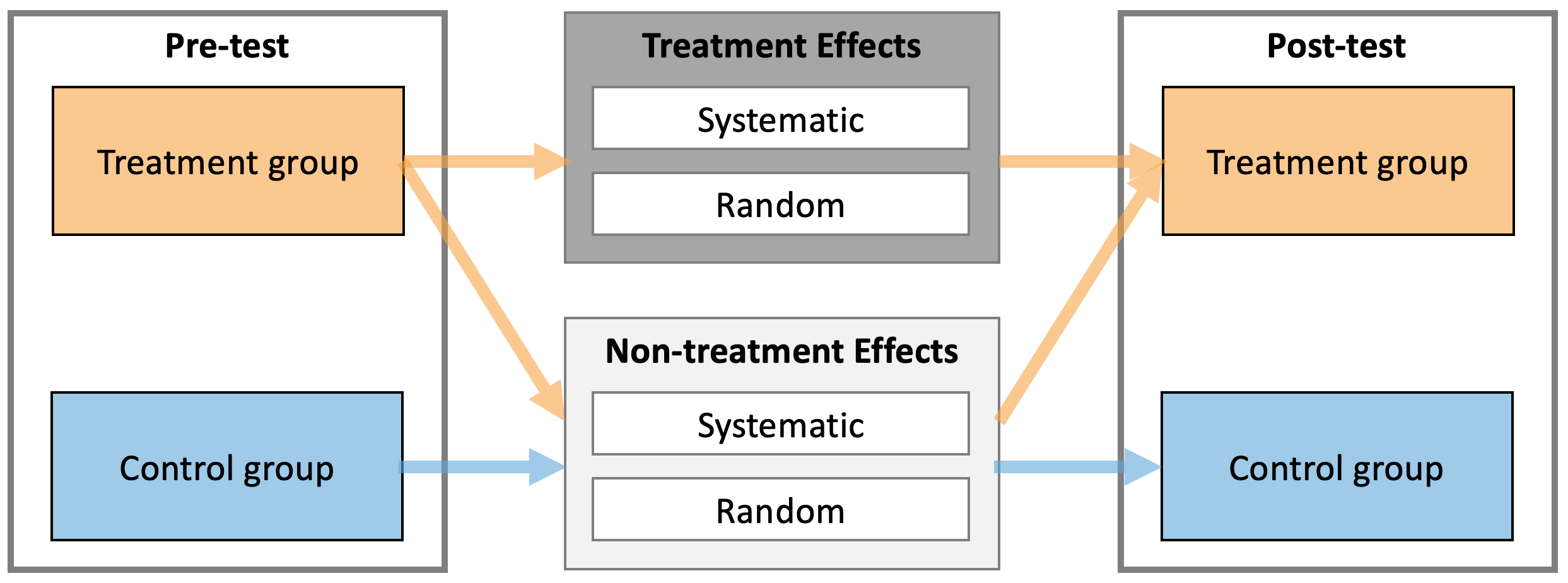
Let’s consider the following RCT DGP. We have two group (Control and Treatment), each with N=10 athletes, measured twice (Pre-test and Post-test) on the vertical jump height, using a measuring device with a known measurement error (i.e. only instrumentation noise; see Validity and Reliability chapter for more info) estimated through validity and reliability studies and equal to 0.5cm. Control group are doing their normal training for 4 weeks, while Treatment group is doing EMS stimulation of their calf muscles on top of their normal training.
Since this is DGP, we will assume there is no treatment effect nor non-treatment effects. Both Control and Treatment groups will experience normal biological variation in their jump height, which is equal to 1.5cm. Please refer to Validity and Reliability chapter for more info about the concepts of true score and measurement error. SESOI for the measured score will be ±5cm (since there is no proportional bias in the measurement, this will also be SESOI for the true score - see Validity and Reliability chapter for more information).
require(tidyverse)
require(bmbstats)
require(cowplot)

set.seed(1667)

n_subjects <- 20


instrumentation_noise <- 0.5
biological_variation <- 1.5

# -------------------------
# Treatment effect
treatment_systematic <- 0
treatment_random <- 0

# Non-treatment effect
non_treatment_systematic <- 0
non_treatment_random <- 0
#-------------------------

RCT_data <- tibble(
  Athlete = paste(
    "Athlete",
    str_pad(
      string = seq(1, n_subjects),
      width = 2,
      pad = "0"
    )
  ),
  Group = rep(c("Treatment", "Control"), length.out = n_subjects),

  # True score
  True_score.Pre = rnorm(n_subjects, 45, 5),

  # Treatment effect
  Treatment_effect = rnorm(
    n = n_subjects,
    mean = treatment_systematic,
    sd = treatment_random),

  Non_treatment_effect = rnorm(
    n = n_subjects,
    mean = non_treatment_systematic,
    sd = non_treatment_random),

  # Calculate the change in true score
  True_score.Change = if_else(
    Group == "Treatment",
    # Treatment group is a sum of treatment and non-treatment effects
    Treatment_effect + Non_treatment_effect,
    # While control group only get non-treatment effects
    Non_treatment_effect
  ),
  True_score.Post = True_score.Pre + True_score.Change,

  # Manifested score
  Manifested_score.Pre = True_score.Pre +
    rnorm(n_subjects, 0, biological_variation),

  Manifested_score.Post = True_score.Post +
    rnorm(n_subjects, 0, biological_variation),

  Manifested_score.Change = Manifested_score.Post -
    Manifested_score.Pre,

  # Measured score
  Measured_score.Pre = Manifested_score.Pre +
    rnorm(n_subjects, 0, instrumentation_noise),

  Measured_score.Post = Manifested_score.Post +
    rnorm(n_subjects, 0, instrumentation_noise),

  Measured_score.Change = Measured_score.Post -
    Measured_score.Pre
)

# Make sure that the Group column is a factor
# This will not create issues with PDP+ICE and ICE plotting later
RCT_data$Group <- factor(RCT_data$Group)

head(RCT_data)
#> # A tibble: 6 x 13
#>   Athlete Group True_score.Pre Treatment_effect Non_treatment_e… True_score.Chan…
#>   <chr>   <fct>          <dbl>            <dbl>            <dbl>            <dbl>
#> 1 Athlet… Trea…           52.9                0                0                0
#> 2 Athlet… Cont…           42.4                0                0                0
#> 3 Athlet… Trea…           49.2                0                0                0
#> 4 Athlet… Cont…           44.8                0                0                0
#> 5 Athlet… Trea…           40.0                0                0                0
#> 6 Athlet… Cont…           42.6                0                0                0
#> # … with 7 more variables: True_score.Post <dbl>, Manifested_score.Pre <dbl>,
#> #   Manifested_score.Post <dbl>, Manifested_score.Change <dbl>, Measured_score.Pre <dbl>,
#> #   Measured_score.Post <dbl>, Measured_score.Change <dbl>
Since we have generated this data, we know that there are no treatment nor non-treatment effects (neither systematic, nor random or variable effects). But let’s plot the data.
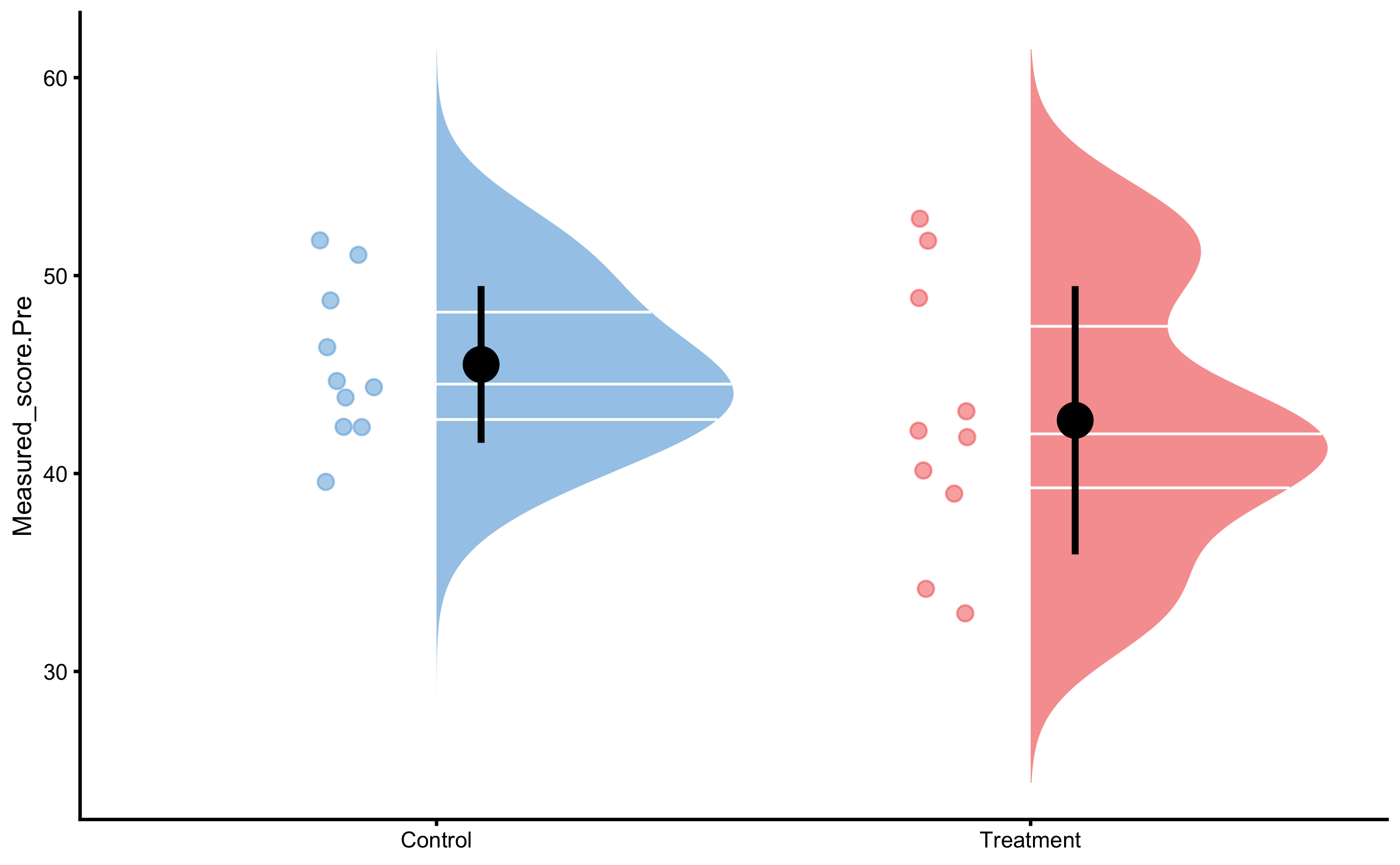
First let’s plot the Pre-test measured scores (vertical jump) distribution:
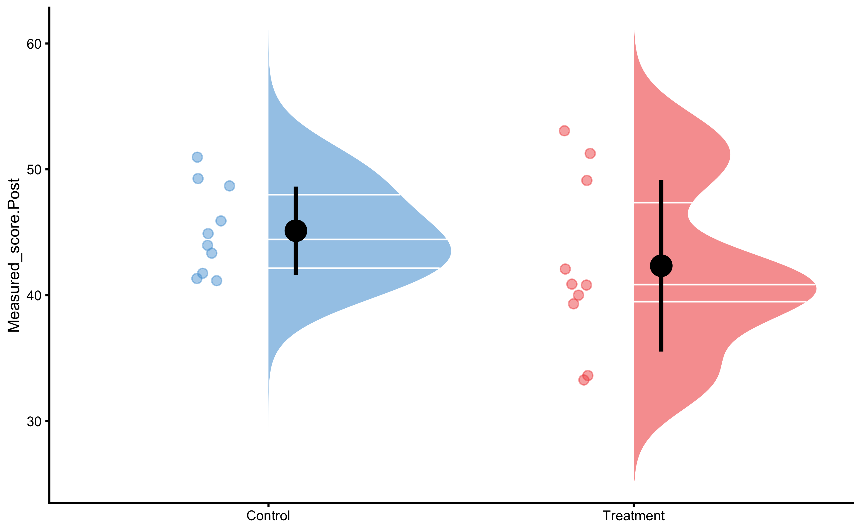
And the Post-test:
And finally measured change scores:
bmbstats::plot_raincloud_SESOI(
  RCT_data,
  value = "Measured_score.Change",
  groups = "Group",
  SESOI_lower = -5,
  SESOI_upper = 5
)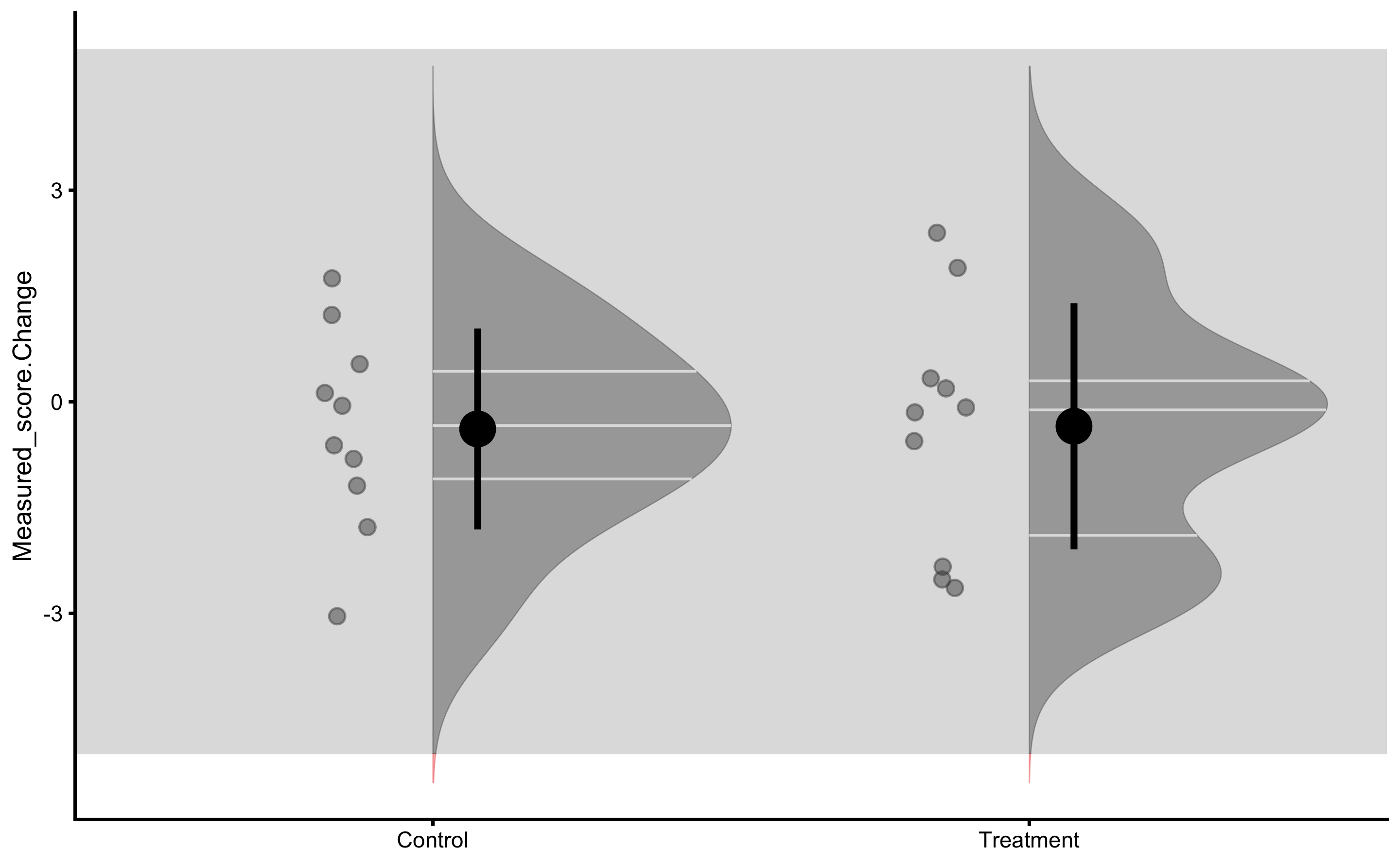
From these graphs we can see that there is no difference between group. We have also selected large SESOI taking into account our a priori knowledge about biological variation and measurement error in the vertical jump height.
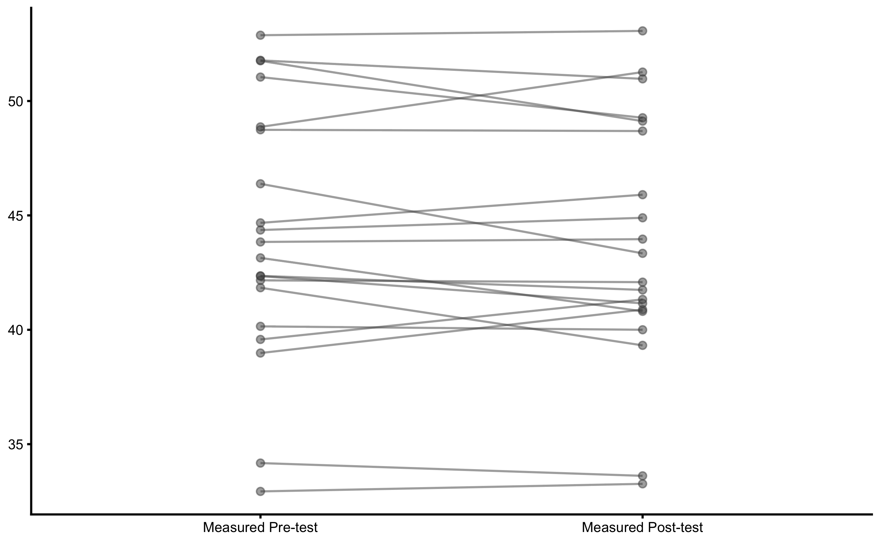
Let’s plot the individual change fro athletes from the Treatment group:
bmbstats::plot_pair_changes(
  group_a = RCT_data$Measured_score.Pre,
  group_b = RCT_data$Measured_score.Post,
  group_a_label = "Measured Pre-test",
  group_b_label = "Measured Post-test",
  SESOI_lower = -5,
  SESOI_upper = 5
)
16.2 RCT analysis using bmbstats::RCT_analysis function
To perform RCT analysis explained in the Causal inference chapter, we will use bmbstats::RCT_analysis function. bmbstats::RCT_analysis function has three built-in estimator function: bmbstats::RCT_estimators, bmbstats::RCT_estimators_simple, and bmbstats::RCT_estimators_lm. bmbstats::RCT_estimators is more extensive and involves individual group analysis, while the bmbstats::RCT_estimators_simple only provides estimated treatment and non-treatment effects. bmbstats::RCT_estimators_lm will be explained in the next section.
extensive_RCT <- bmbstats::RCT_analysis(
  data = RCT_data,
  group = "Group",
  treatment_label = "Treatment",
  control_label = "Control",
  pre_test = "Measured_score.Pre",
  post_test = "Measured_score.Post",
  SESOI_lower = -5,
  SESOI_upper = 5,
  control = model_control(seed = 1667)
)
#> [1] "All values of t are equal to  5 \n Cannot calculate confidence intervals"
#> [1] "All values of t are equal to  10 \n Cannot calculate confidence intervals"


extensive_RCT
#> Bootstrap with 2000 resamples and 95% bca confidence intervals.
#>
#>                           estimator         value         lower        upper
#>                         SESOI lower -5.0000000000            NA           NA
#>                         SESOI upper  5.0000000000            NA           NA
#>                         SESOI range 10.0000000000            NA           NA
#>         Control Group Pre-test mean 45.5109521606  4.338522e+01  47.99500924
#>           Control Group Pre-test SD  3.9597464864  2.821249e+00   5.39401519
#>        Control Group Post-test mean 45.1257775214  4.327530e+01  47.33738237
#>          Control Group Post-test SD  3.5092078780  2.612392e+00   4.59657735
#>       Treatment Group Pre-test mean 42.6896373231  3.878113e+01  46.84572579
#>         Treatment Group Pre-test SD  6.7766398945  4.783839e+00   8.92052081
#>      Treatment Group Post-test mean 42.3426726375  3.856045e+01  46.63546378
#>        Treatment Group Post-test SD  6.8172485979  4.880090e+00   8.96710016
#>                  Pre-test pooled SD  5.5498847059  4.348937e+00   7.08556923
#>           Pre-test Group difference -2.8213148375 -7.362312e+00   1.66624873
#>          Post-test Group difference -2.7831048839 -7.151974e+00   1.84048180
#>           Control Group Change mean -0.3851746392 -1.301390e+00   0.35428624
#>             Control Group Change SD  1.4244343846  9.592800e-01   2.04852176
#>             Control Group Cohen's d -0.0694022776 -2.627647e-01   0.08120665
#>       Control Group Change to SESOI -0.0385174639 -1.301390e-01   0.03542862
#>    Control Group Change SD to SESOI  0.1424434385  9.592800e-02   0.20485218
#>                Control Group pLower  0.0050812820  3.123715e-04   0.04282747
#>           Control Group pEquivalent  0.9927461183  9.564951e-01   0.99950198
#>               Control Group pHigher  0.0021725997  2.037526e-04   0.01324039
#>         Treatment Group Change mean -0.3469646855 -1.363329e+00   0.72633527
#>           Treatment Group Change SD  1.7452275994  1.230571e+00   2.23150783
#>           Treatment Group Cohen's d -0.0625174583 -2.845506e-01   0.16106127
#>     Treatment Group Change to SESOI -0.0346964686 -1.363329e-01   0.07263353
#>  Treatment Group Change SD to SESOI  0.1745227599  1.230571e-01   0.22315078
#>              Treatment Group pLower  0.0128923459  1.224420e-03   0.03986666
#>         Treatment Group pEquivalent  0.9803630085  9.469588e-01   0.99789556
#>             Treatment Group pHigher  0.0067446456  6.592220e-04   0.03469121
#>                    Effect Cohen's d  0.0268246499 -1.142476e+00   1.10911957
#>                   Systematic effect  0.0382099536 -1.239017e+00   1.40527411
#>                       Random effect  1.0083680171 -1.142340e+00   1.85676617
#>          Systematic effect to SESOI  0.0038209954 -1.239017e-01   0.14052741
#>              SESOI to Random effect  9.9170142553 -1.104973e+01 149.46811634
#>                              pLower  0.0003713043  1.345150e-12   0.99988780
#>                         pEquivalent  0.9992167407 -9.960108e-01   1.00000000
#>                             pHigher  0.0004119550  1.014997e-12   0.99983149
We can also plot the estimators bootstrap distributions:
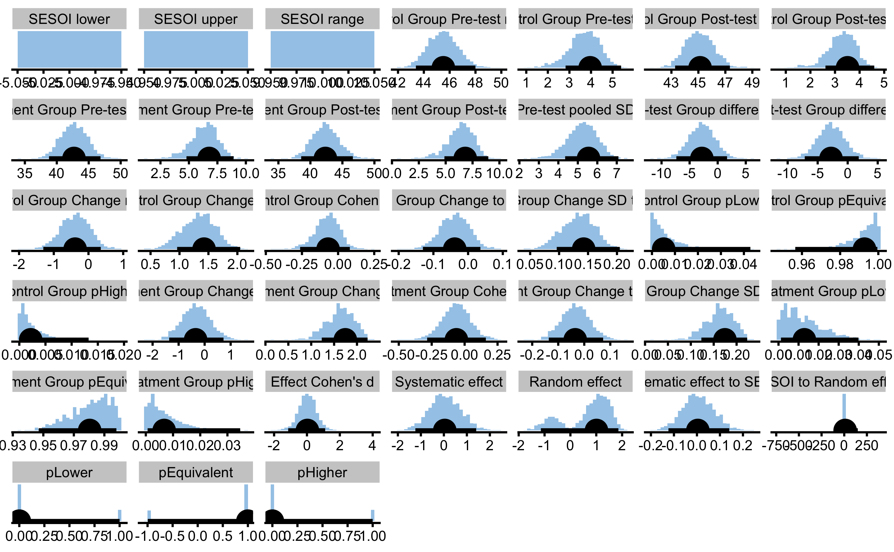
If we use bmbstats::RCT_estimators_simple, we will get much more condensed output:
simple_RCT <- bmbstats::RCT_analysis(
  data = RCT_data,
  group = "Group",
  treatment_label = "Treatment",
  control_label = "Control",
  pre_test = "Measured_score.Pre",
  post_test = "Measured_score.Post",
  SESOI_lower = -5,
  SESOI_upper = 5,
  estimator_function = bmbstats::RCT_estimators_simple,
  control = model_control(seed = 1667)
)
#> [1] "All values of t are equal to  5 \n Cannot calculate confidence intervals"
#> [1] "All values of t are equal to  10 \n Cannot calculate confidence intervals"


simple_RCT
#> Bootstrap with 2000 resamples and 95% bca confidence intervals.
#>
#>                   estimator         value         lower       upper
#>                 SESOI lower -5.0000000000            NA          NA
#>                 SESOI upper  5.0000000000            NA          NA
#>                 SESOI range 10.0000000000            NA          NA
#>           Systematic effect  0.0382099536 -1.239017e+00   1.4052741
#>               Random effect  1.0083680171 -1.142340e+00   1.8567662
#>  Systematic effect to SESOI  0.0038209954 -1.239017e-01   0.1405274
#>      SESOI to Random effect  9.9170142553 -1.104973e+01 149.4681163
#>                      pLower  0.0003713043  1.345150e-12   0.9998878
#>                 pEquivalent  0.9992167407 -9.960108e-01   1.0000000
#>                     pHigher  0.0004119550  1.014997e-12   0.9998315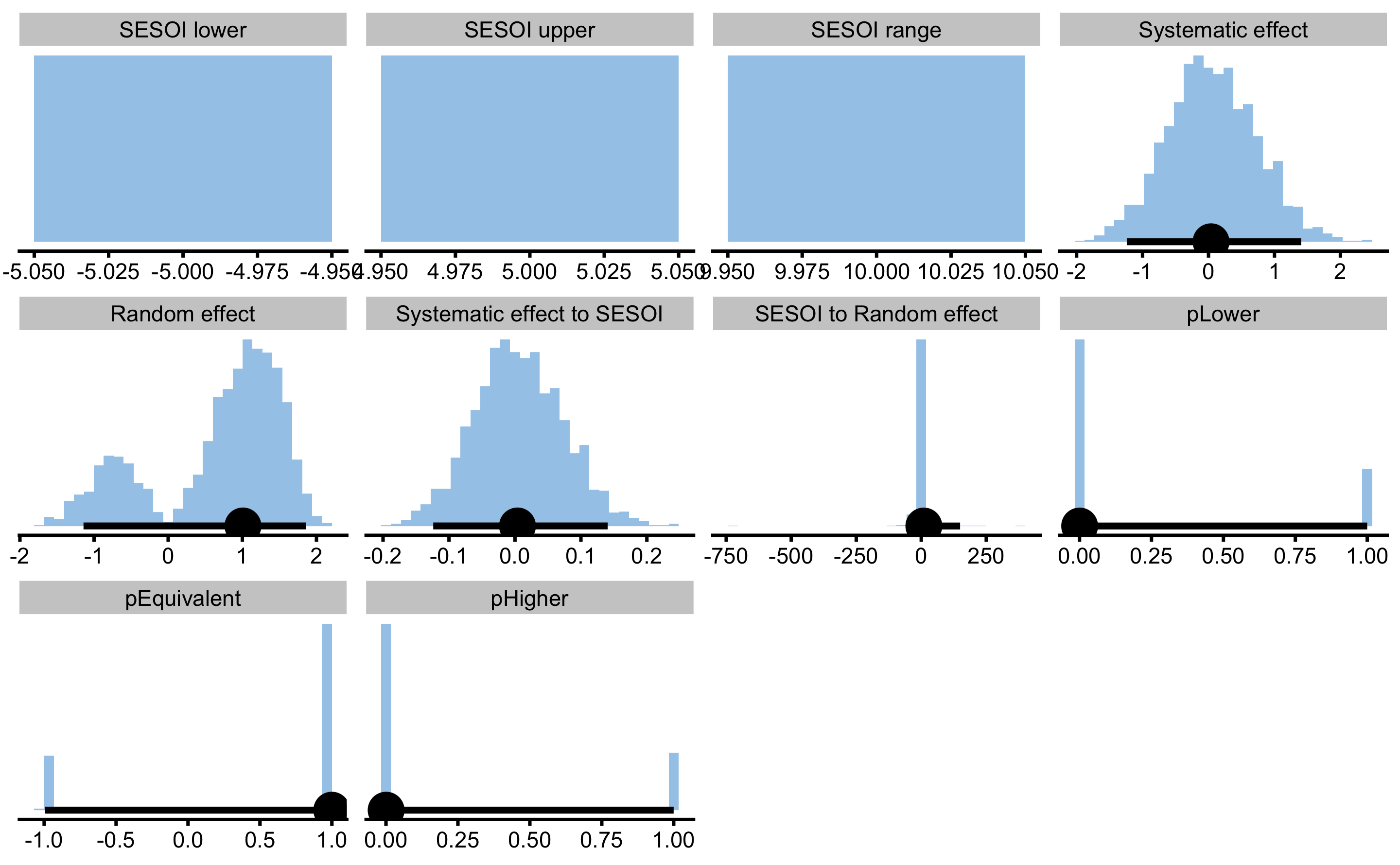
As can be seen, the analysis correctly identified no treatment effect. There is an issue with random treatment effects estimation since is demonstrates distribution with two peaks. This effect is due to random treatment effect being zero and the way the root of the squared differences is calculated to avoid irrational numbers (i.e. taking root of negative number).
There are additional graphs that can be produced. All graphs can take control = plot_control parameter to setup plotting options as explained in the previous chapters.
Control group Pre- and Post-test distribution:
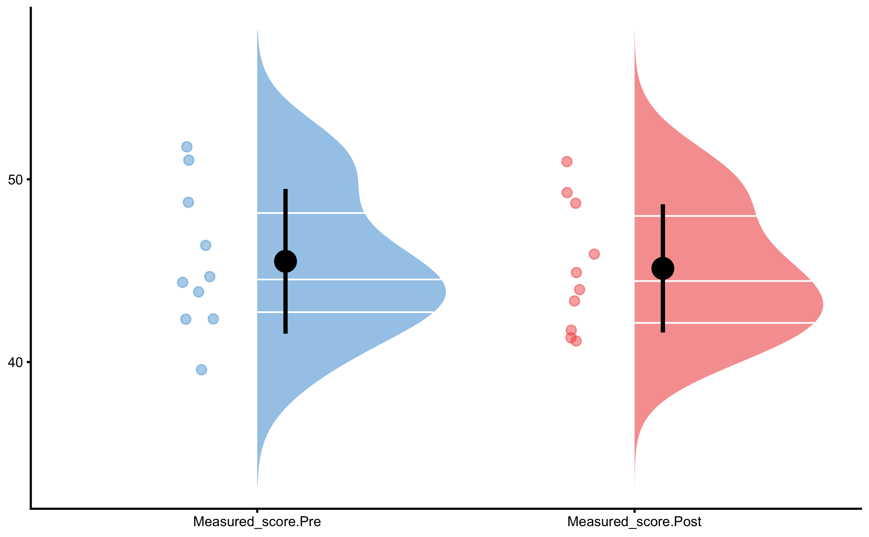
Treatment group Pre- and Post-test distribution:
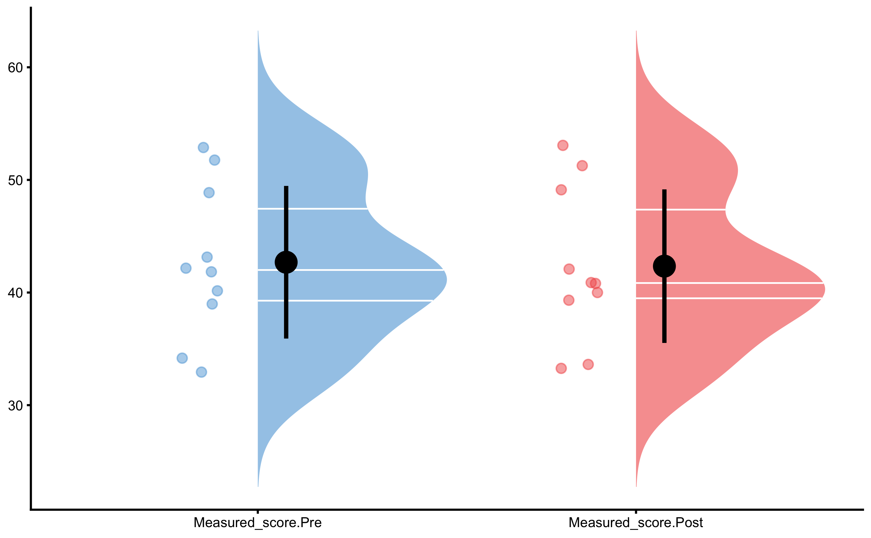
Control change graph:
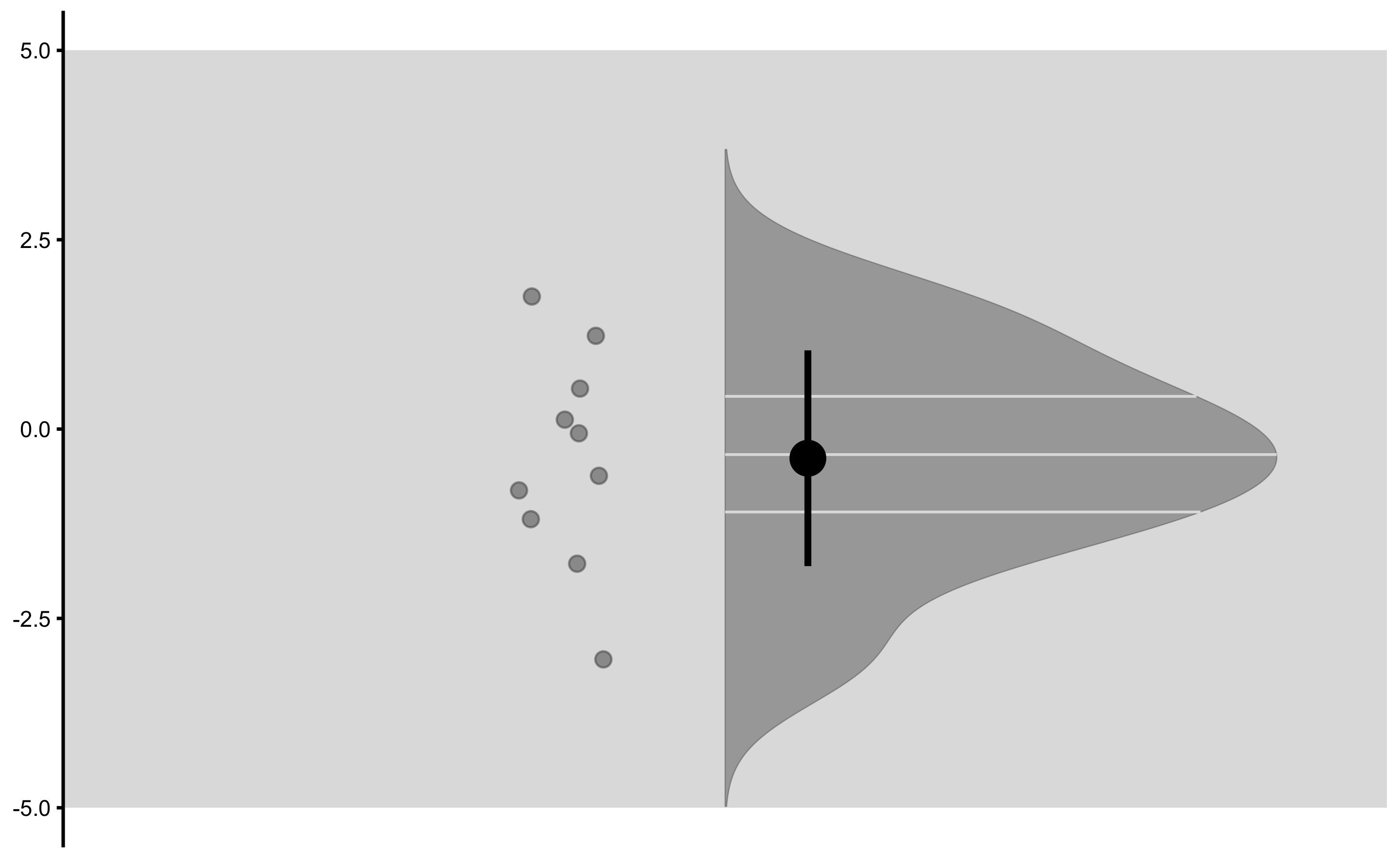
Treatment change graph:
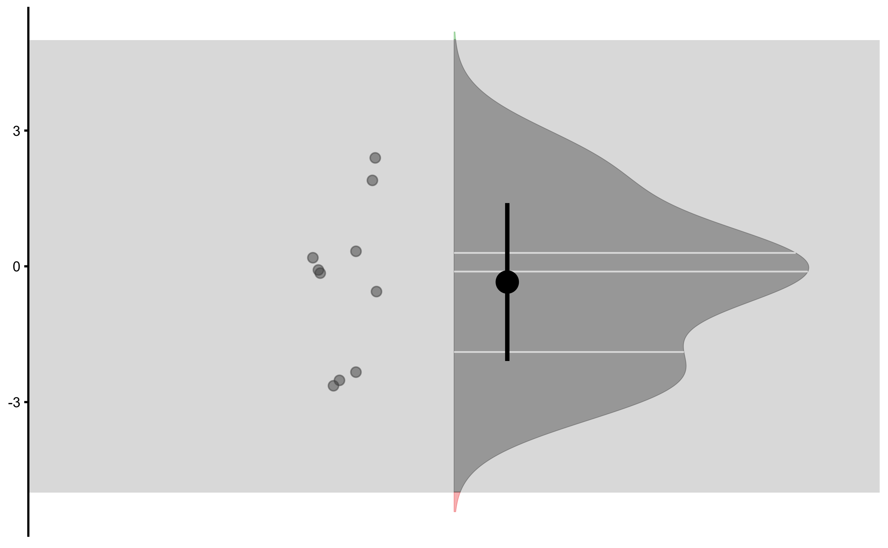
Change graph:
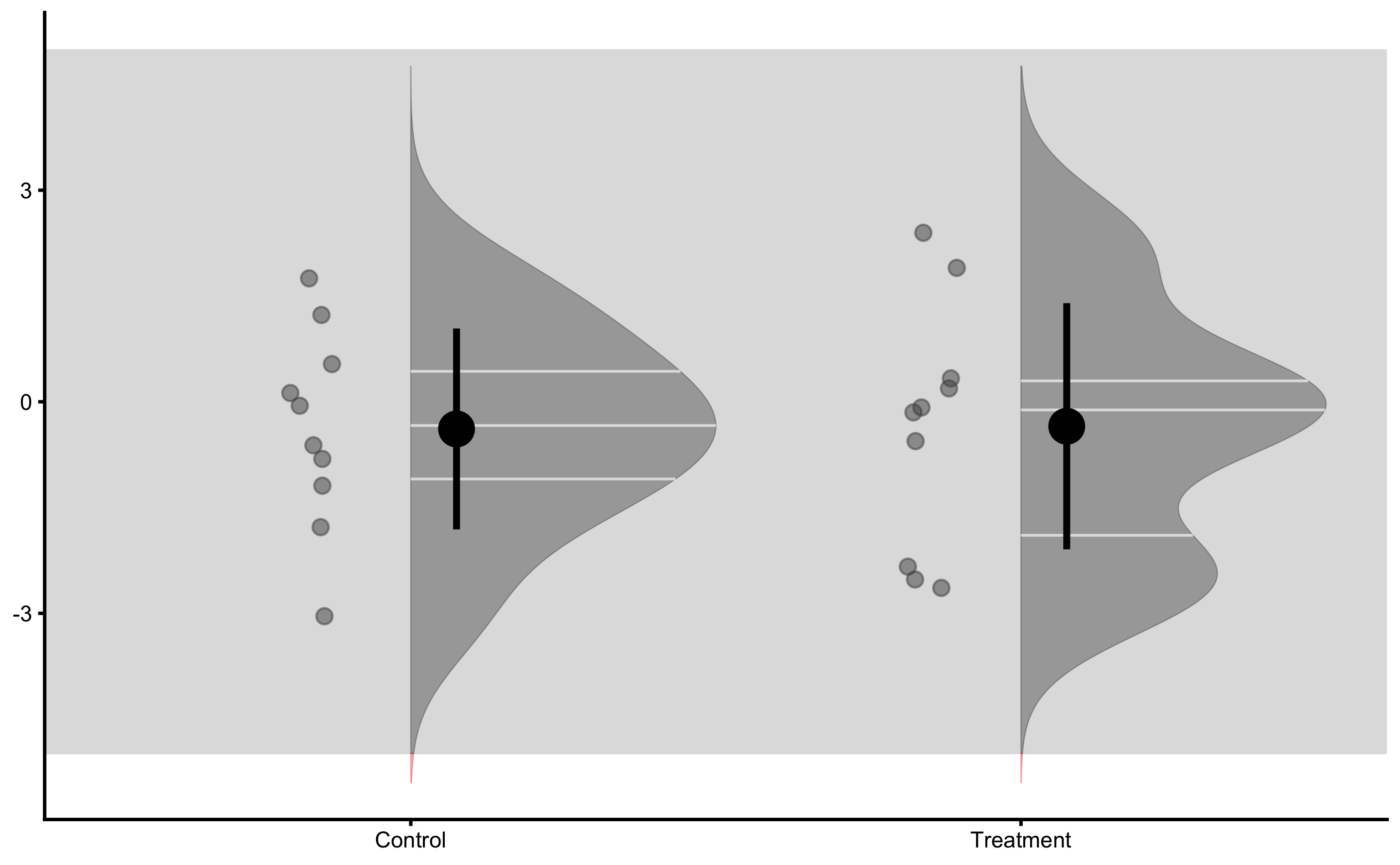
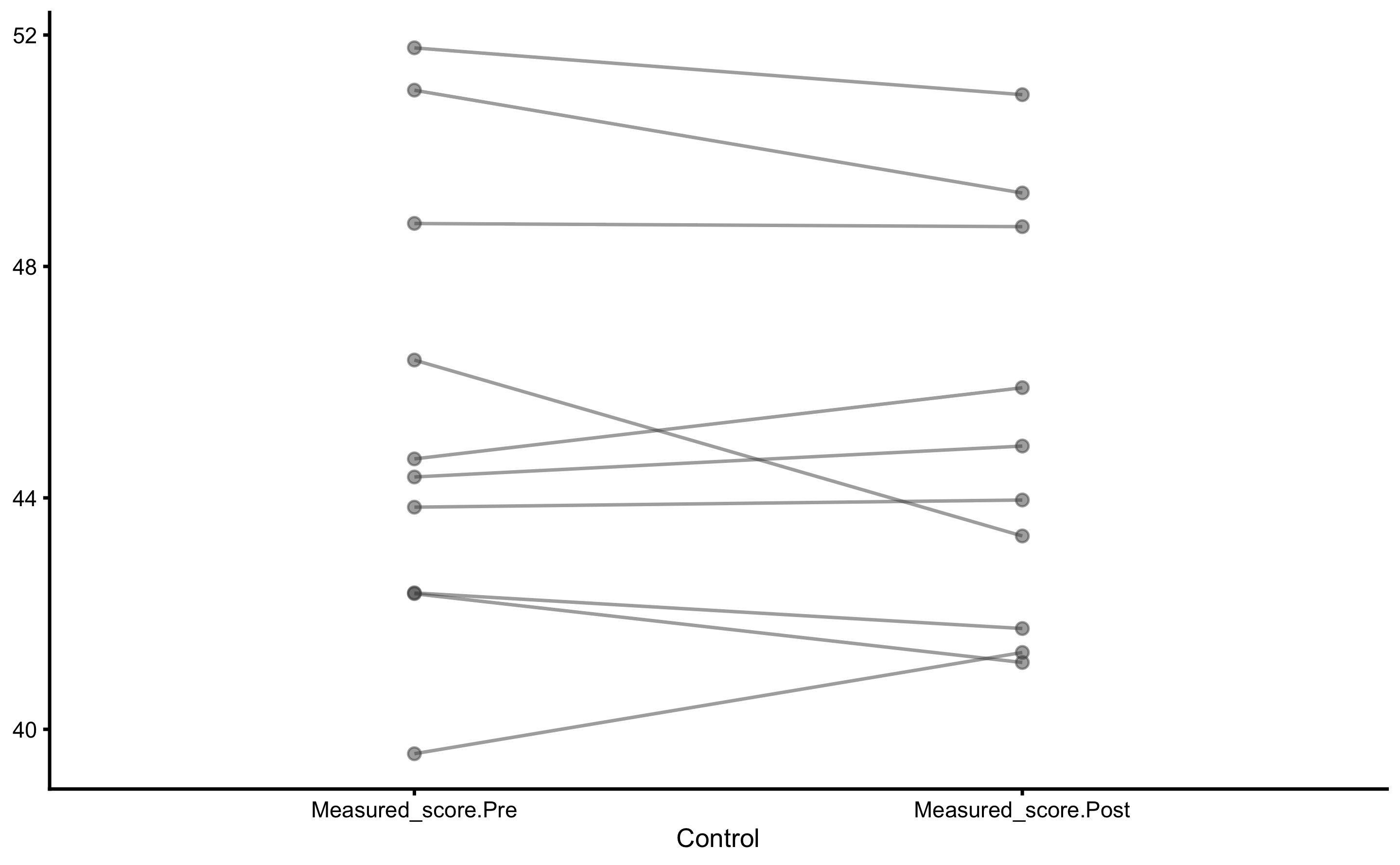
Individual changes in the Control group:
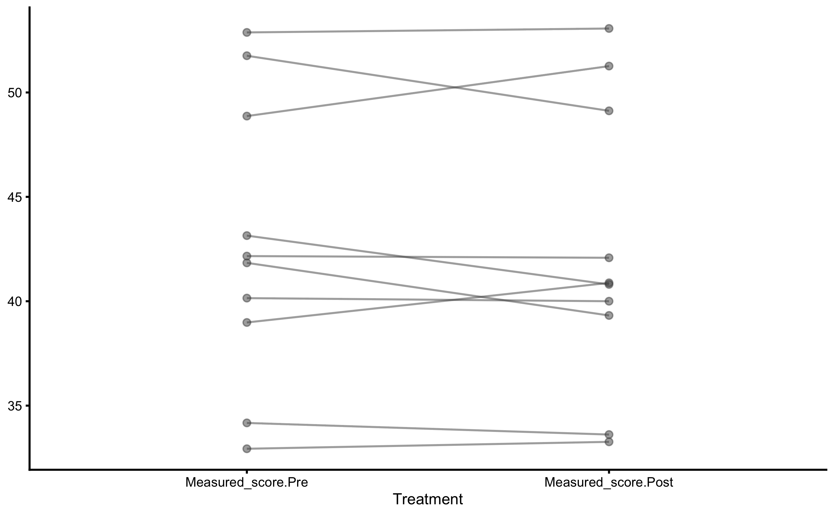
Individual changes in the Treatment group:
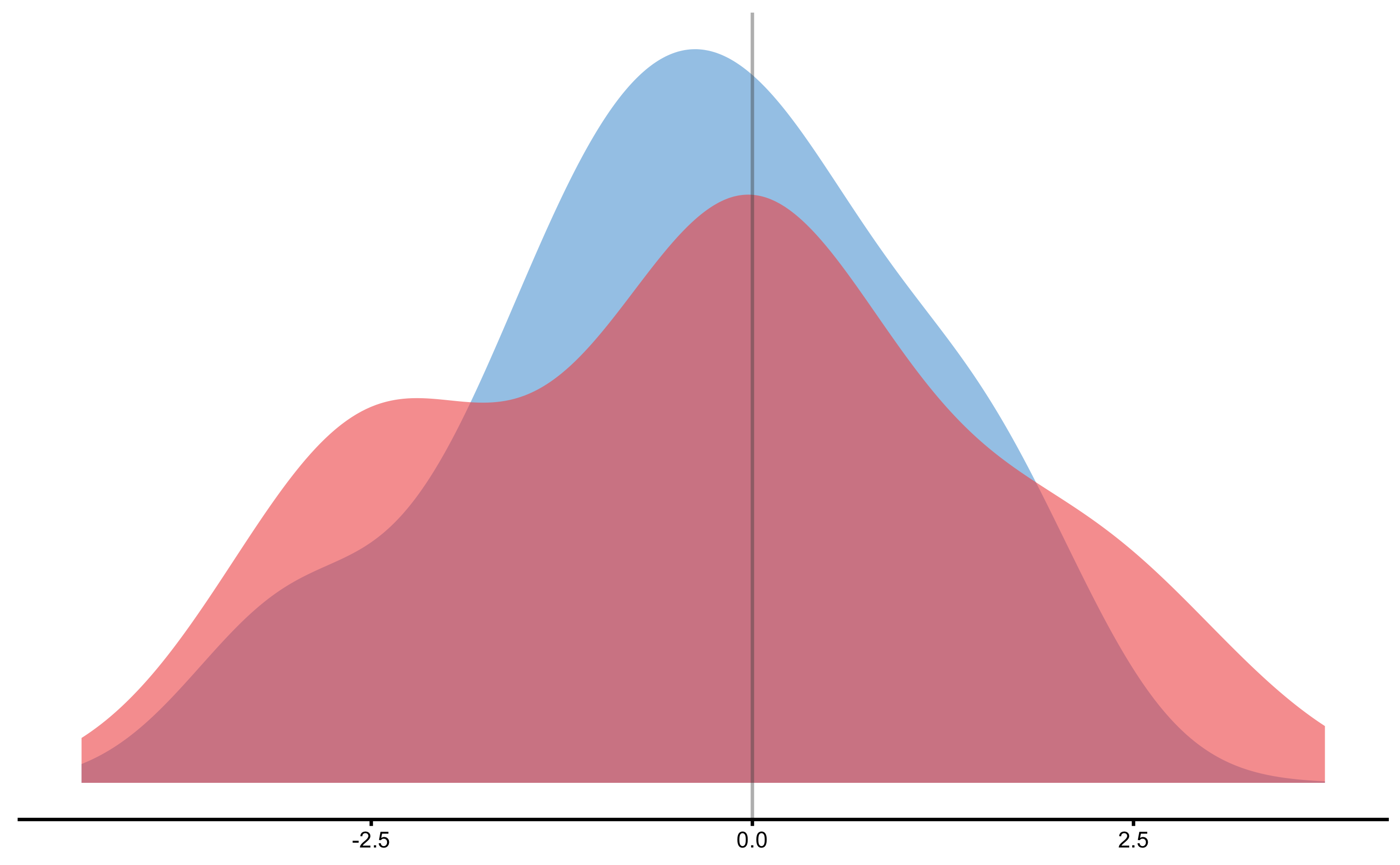
Distribution of the change scores:
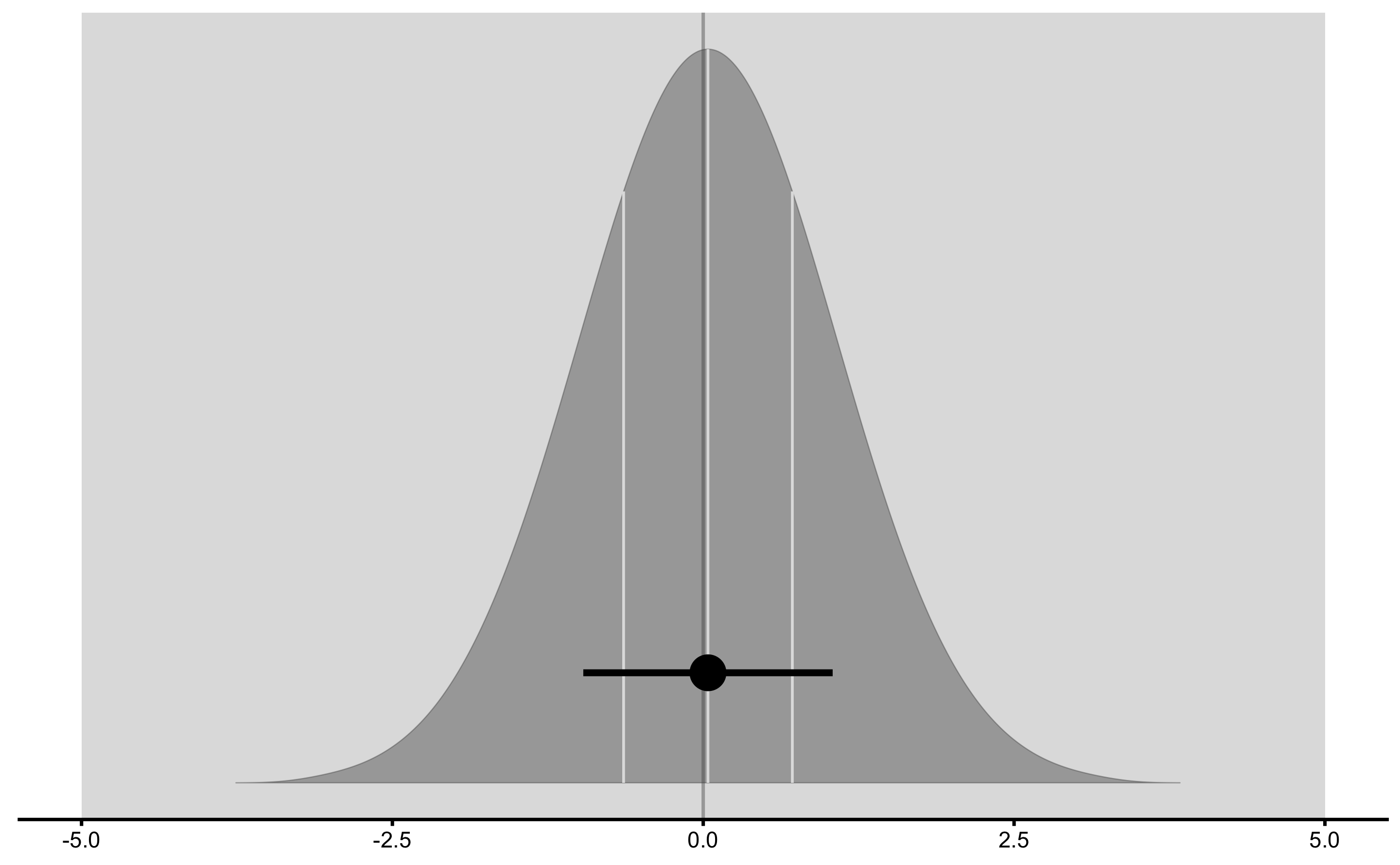
Treatment effect distribution:
And finally, adjusted treatment responses:
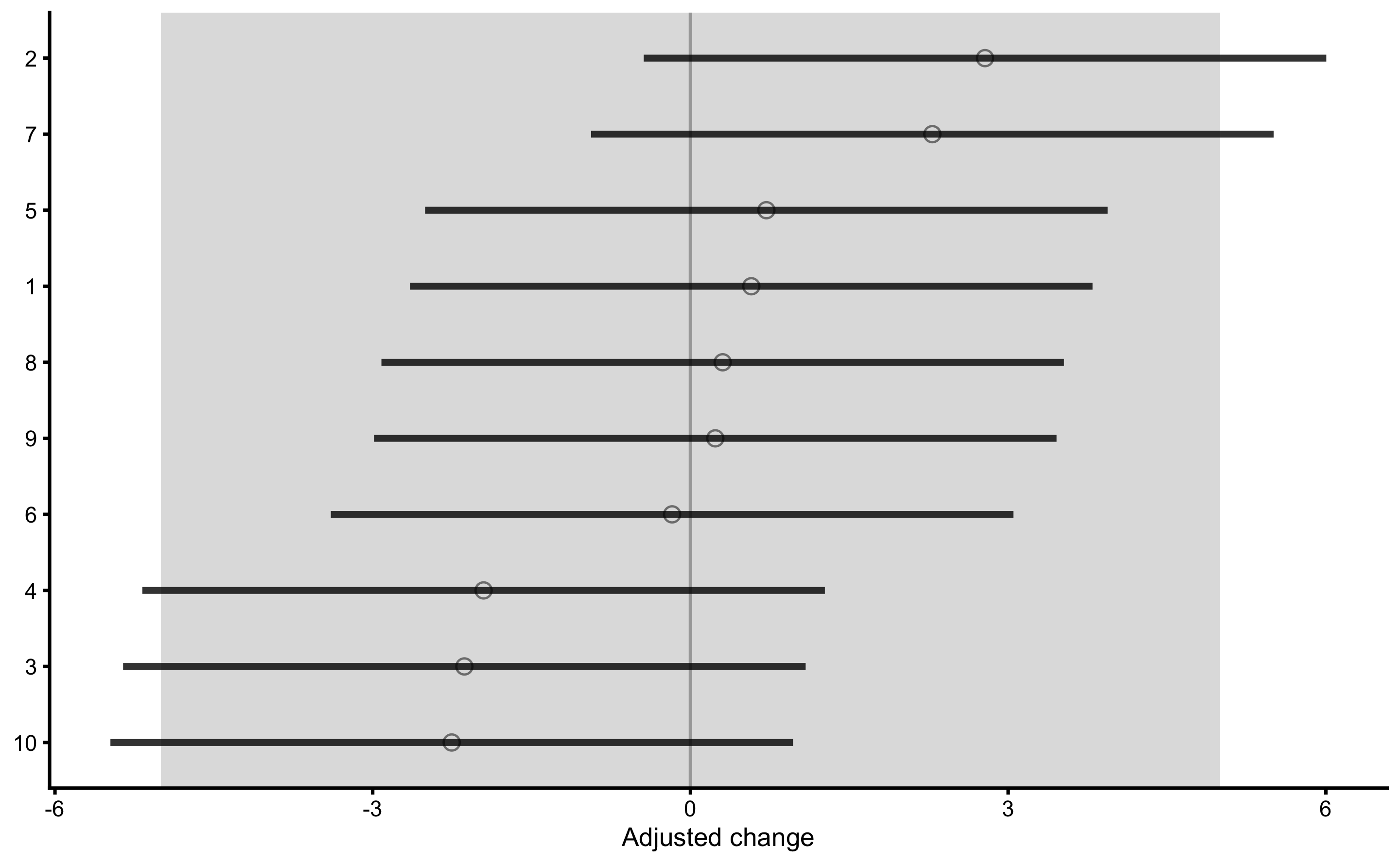
The adjusted treatment responses are calculated by deducting mean Control group change from individual change in the Treatment group (i.e. adjusted change). Error-bars represent 95% confidence intervals (i.e. SDC) using change SD of the Control group.
The data used to create this graph can be found in the returned object:
head(simple_RCT$extra$treatment_responses)
#>    id     group pre_test post_test     change      SDC change_lower change_upper
#> 11  1 Treatment 52.87665  53.06613  0.1894841 3.222294   -3.0328104    3.4117785
#> 12  2 Treatment 48.86917  51.26538  2.3962116 3.222294   -0.8260828    5.6185061
#> 13  3 Treatment 41.83908  39.31947 -2.5196029 3.222294   -5.7418974    0.7026915
#> 14  4 Treatment 43.14467  40.80646 -2.3382079 3.222294   -5.5605023    0.8840866
#> 15  5 Treatment 32.93471  33.26669  0.3319806 3.222294   -2.8903138    3.5542751
#> 16  6 Treatment 34.17358  33.61544 -0.5581425 3.222294   -3.7804369    2.6641520
#>    adjusted_change adjusted_change_lower adjusted_change_upper
#> 11       0.5746587            -2.6476357              3.796953
#> 12       2.7813863            -0.4409082              6.003681
#> 13      -2.1344283            -5.3567227              1.087866
#> 14      -1.9530332            -5.1753277              1.269261
#> 15       0.7171553            -2.5051392              3.939450
#> 16      -0.1729678            -3.3952623              3.049327
We can also plot the un-adjusted treatment responses:
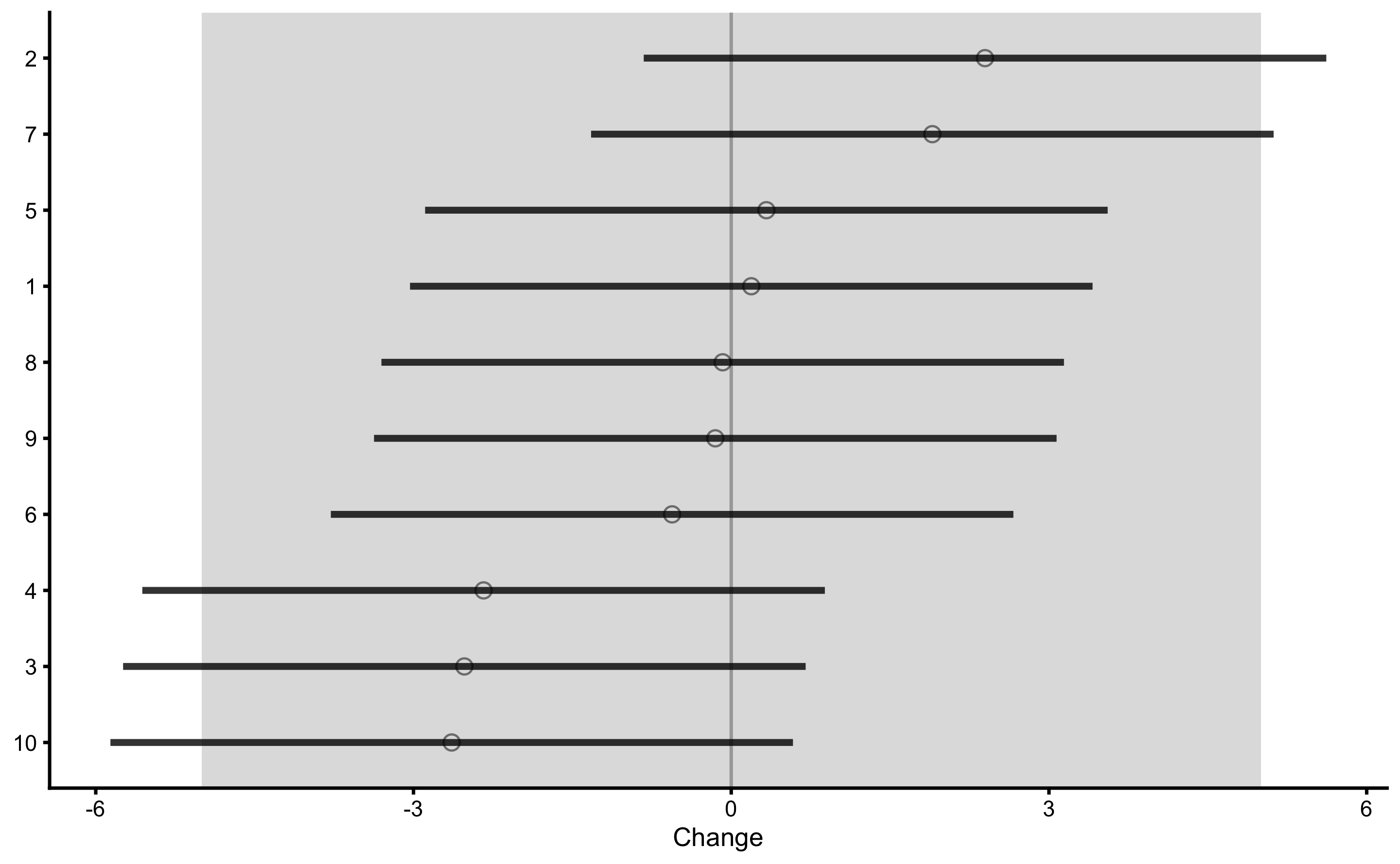
Let’s re-create this graph using bmbstats::observations_MET function since that function also allows us to set Type I error rates and confidence for plotting.
treatment_group <- filter(
  RCT_data,
  Group == "Treatment"
)

control_group <- filter(
  RCT_data,
  Group == "Control"
)

treatment_responses <- bmbstats::observations_MET(
  observations = treatment_group$Measured_score.Change -
    mean(control_group$Measured_score.Change),

  observations_label = treatment_group$Athlete,

  # Use control group change as measurement error
  measurement_error = sd(control_group$Measured_score.Change),

  # Degrees of freedom from the reliability study. Use `Inf` for normal distribution
  df = nrow(control_group) - 1,
  SESOI_lower = -5,
  SESOI_upper = 5,

  # Will not use Bonferroni adjustment here
  alpha = 0.05,
  # No adjustment in CIs for plotting
  confidence = 0.95
)

plot(
  treatment_responses,
  true_observations = treatment_group$True_score.Change,
  control = plot_control(points_size = 5)
) +
  xlim(-9, 9)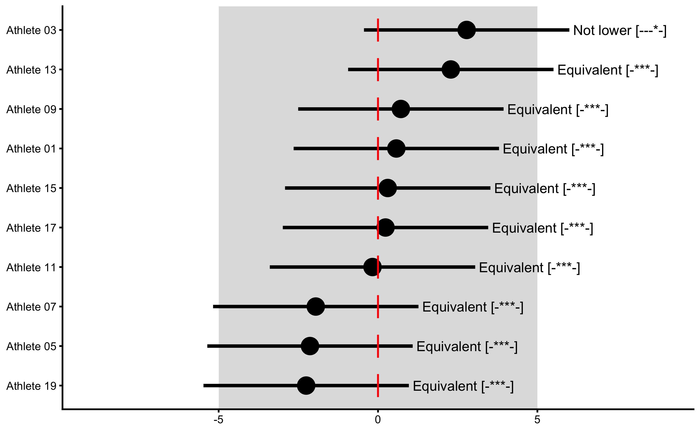
This way, Control group is used as sort-of reliability study (see Repeatability section in the Validity and Reliability chapter) that provides source of information about the non-treatment effect (in this case 0 for both systematic and random components), biological variation and instrumentation noise. This helps us to provide uncertainty intervals around individual treatment (adjusted) effects.
16.3 Linear Regression Perspective
RCT analysis performed with bmbstats::RCT_analysis is the method of differences (i.e. changes). This is similar to the method of differences explained in the Validity and Reliability chapter. Another approach is to utilize linear regression( explained in the Prediction as a complement to causal inference section of the Causal inference chapter). To understand this, let’s depict this RCT data by using Group as predictor and Change score as outcome:
ggplot(
  RCT_data,
  aes(x = Group, y = Measured_score.Change, color = Group)
) +
  theme_cowplot(8) +
  geom_jitter(width = 0.2) +
  scale_color_manual(values = c(Treatment = "#FAA43A", Control = "#5DA5DA"))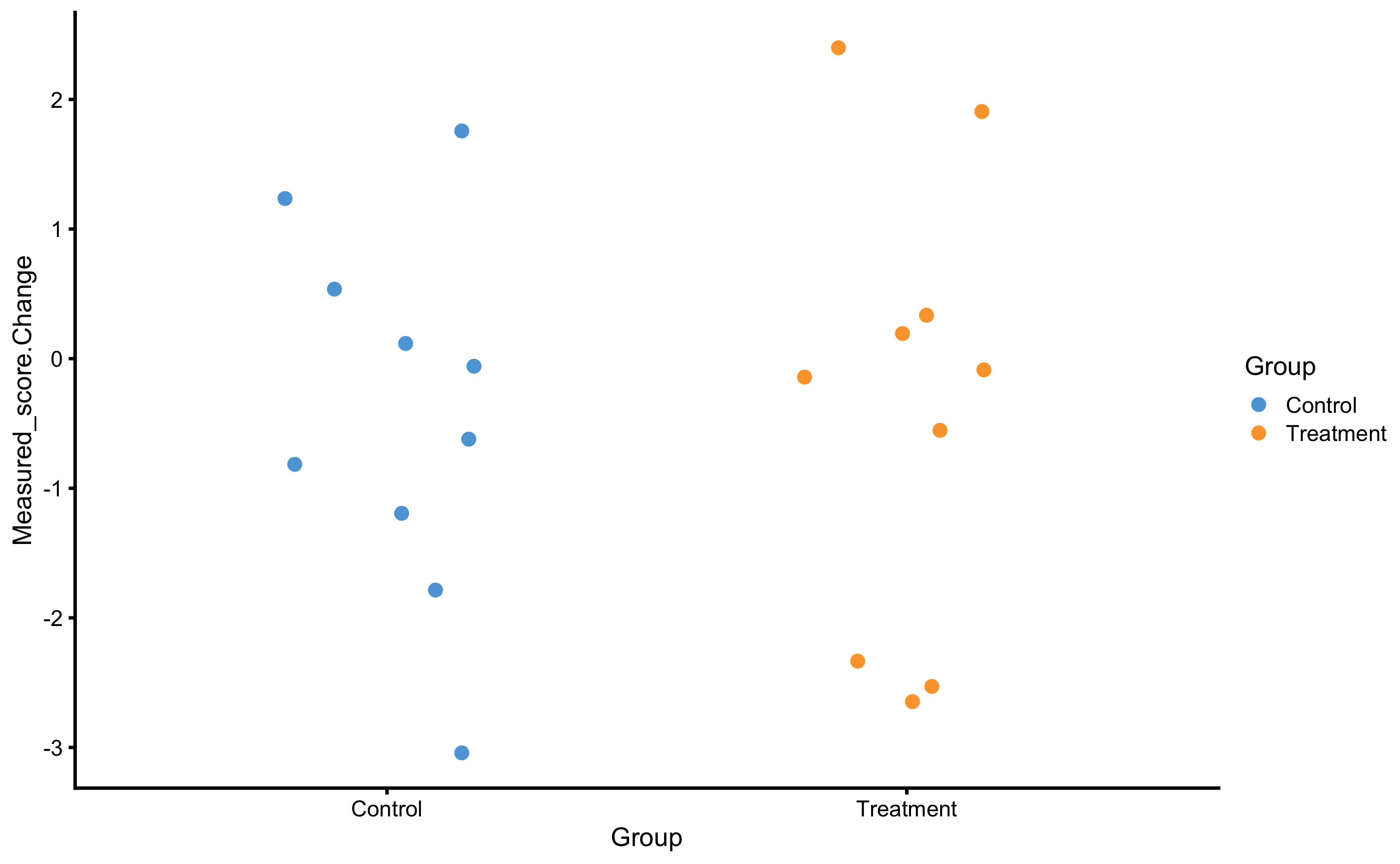
If we perform the linear regression, we will get the following:
model1 <- lm(
  Measured_score.Change ~ Group,
  RCT_data
)

summary(model1)
#>
#> Call:
#> lm(formula = Measured_score.Change ~ Group, data = RCT_data)
#>
#> Residuals:
#>     Min      1Q  Median      3Q     Max
#> -2.6559 -0.9517  0.2315  0.7391  2.7432
#>
#> Coefficients:
#>                Estimate Std. Error t value Pr(>|t|)
#> (Intercept)    -0.38517    0.50373  -0.765    0.454
#> GroupTreatment  0.03821    0.71238   0.054    0.958
#>
#> Residual standard error: 1.593 on 18 degrees of freedom
#> Multiple R-squared:  0.0001598,  Adjusted R-squared:  -0.05539
#> F-statistic: 0.002877 on 1 and 18 DF,  p-value: 0.9578
Intercept in this case (-0.39cm) represents the mean change in the Control group, while slope (GroupTreatment; 0.04cm) represents estimate of the systematic treatment effect (i.e. difference in means).
This can be easily explained visually:
RCT_data$Group_num <- ifelse(
  RCT_data$Group == "Treatment",
  1,
  0
)

ggplot(
  RCT_data,
  aes(x = Group_num, y = Measured_score.Change)
) +
  theme_cowplot(8) +
  geom_jitter(aes(color = Group), width = 0.2) +
  geom_smooth(method = "lm", formula = y ~ x, se = TRUE) +
  scale_color_manual(values = c(Treatment = "#FAA43A", Control = "#5DA5DA")) +
  scale_x_continuous(
    name = "Group",
    breaks = c(0, 1),
    labels = c("Control", "Treatment")
  )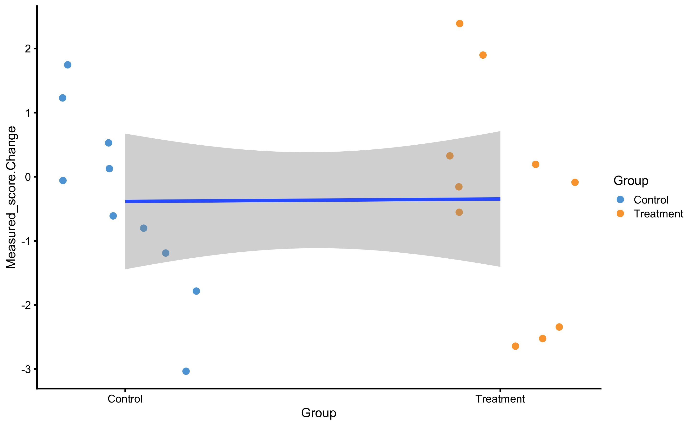
Random components of the treatment and non-treatment effects can be seen as residuals (actually as SD of the residuals) around mean of the group changes. RSE of this model (1.59cm) represents pooled random errors of both Treatment and Control groups. If we perform SD of the residuals for each Group, we will get the following:
SD_summary <- RCT_data %>%
  mutate(.resid = residuals(model1)) %>%
  group_by(Group) %>%
  summarise(`Residual SD` = sd(.resid))

SD_summary
#> # A tibble: 2 x 2
#>   Group     `Residual SD`
#>   <fct>             <dbl>
#> 1 Control            1.42
#> 2 Treatment          1.75
Estimating random treatment effect is thus equal to: \[\begin{equation} \sqrt{SD_{Treatment \;group}^2 - SD_{Control \; group}^2} \end{equation}\]
If you compare these regression estimates to those from the bmbstats::RCT_analysis, you will notice they are equal.
But, as alluded in Causal inference chapter, one should avoid using Change scores and rather use Pre-test and Post-test scores. In this case, our model would look visually like this (I have added dashed identity line so Pre-test and Post-test comparison is easier):
ggplot(
  RCT_data,
  aes(x = Measured_score.Pre, y = Measured_score.Post, color = Group, fill = Group)
) +
  theme_cowplot(8) +
  geom_abline(slope = 1, linetype = "dashed") +
  geom_smooth(method = "lm", se = TRUE, alpha = 0.2) +
  geom_point(alpha = 0.8) +
  scale_color_manual(values = c(Treatment = "#FAA43A", Control = "#5DA5DA")) +
  scale_fill_manual(values = c(Treatment = "#FAA43A", Control = "#5DA5DA"))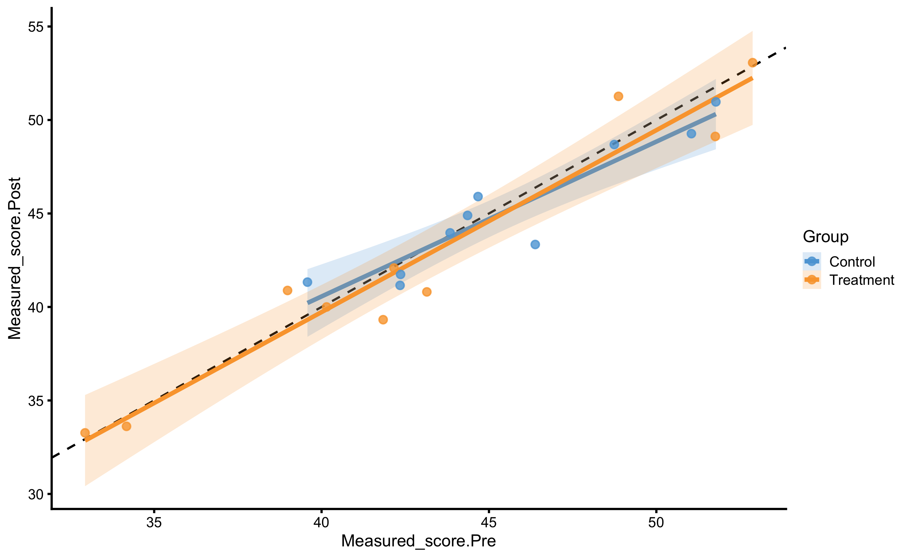
And estimated linear regression model:
model2 <- lm(
  Measured_score.Post ~ Measured_score.Pre + Group,
  RCT_data
)

summary(model2)
#>
#> Call:
#> lm(formula = Measured_score.Post ~ Measured_score.Pre + Group,
#>     data = RCT_data)
#>
#> Residuals:
#>      Min       1Q   Median       3Q      Max
#> -2.60014 -1.01512  0.04426  0.93174  3.13880
#>
#> Coefficients:
#>                    Estimate Std. Error t value Pr(>|t|)
#> (Intercept)         2.52854    3.12937   0.808     0.43
#> Measured_score.Pre  0.93598    0.06786  13.793 1.16e-10 ***
#> GroupTreatment     -0.14242    0.73977  -0.193     0.85
#> ---
#> Signif. codes:  0 '***' 0.001 '**' 0.01 '*' 0.05 '.' 0.1 ' ' 1
#>
#> Residual standard error: 1.598 on 17 degrees of freedom
#> Multiple R-squared:  0.9236, Adjusted R-squared:  0.9146
#> F-statistic: 102.7 on 2 and 17 DF,  p-value: 3.22e-10
In this model, Pre-test represent covariate. The estimated coefficient for this covariate is 0.94, or very close to 1.
The systematic treatment effect (-0.14cm) can be interpreted as “everything else being equal, changing group from Control to Treatment will result in” effect on the Post-test. Graphically, this represent the vertical gap between the two lines. Please note that in the previous graph, each group is modeled separately, and in this model the lines are assumed to be parallel (i.e. no interaction between the lines - or no interaction between Group and Pre-test). Let us thus plot our model:
RCT_data$.pred <- predict(
  model2,
  newdata = RCT_data
)

ggplot(
  RCT_data,
  aes(x = Measured_score.Pre, y = Measured_score.Post, color = Group, fill = Group)
) +
  theme_cowplot(8) +
  geom_point(alpha = 0.8) +
  geom_line(aes(y = .pred)) +
  scale_color_manual(values = c(Treatment = "#FAA43A", Control = "#5DA5DA")) +
  scale_fill_manual(values = c(Treatment = "#FAA43A", Control = "#5DA5DA"))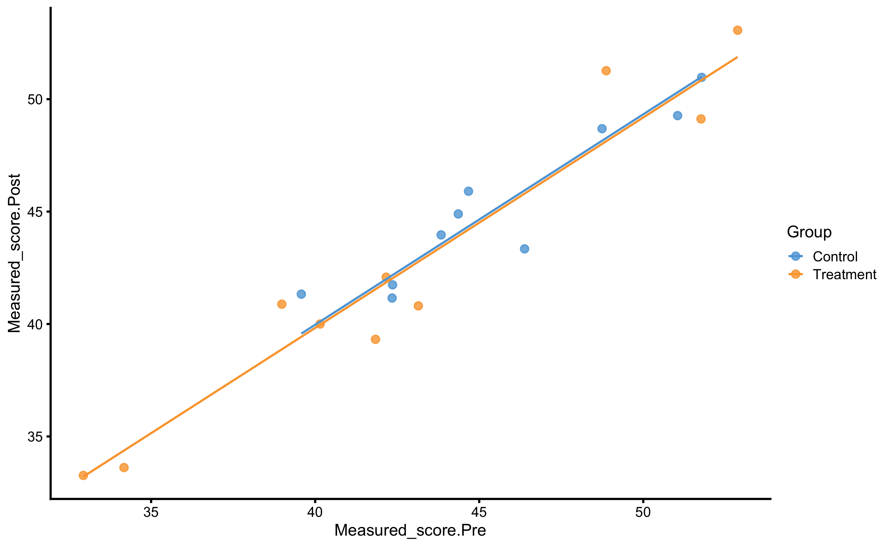
As can be seen from the figure, lines are almost identical, but more importantly, they are now parallel.
To estimate random treatment effect, we can use residuals SD for each group yet again.
SD_summary <- RCT_data %>%
  mutate(.resid = residuals(model2)) %>%
  group_by(Group) %>%
  summarise(`Residual SD` = sd(.resid))

SD_summary
#> # A tibble: 2 x 2
#>   Group     `Residual SD`
#>   <fct>             <dbl>
#> 1 Control            1.32
#> 2 Treatment 1.75This concept was a bit hard for me to wrap my head around as well. Residuals are something we cannot explain with our model (be it using simple mean with the method of differences, or using linear regression model with Group and Pre-test). Everything we can explain with the model can be thus seen as systematic effect. Thus, the thing that is left is unexplained variance. This variance is due to biological variation, instrumentation error and random non-treatment effects (which are zero in this example), as well as random treatment effects (which are also zero in this example).
This approach is implemented in bmbstats::RCT_estimators_lm function that we can use in bmbstats::RCT_analysis to get bootstrap CIs:
regression_RCT <- bmbstats::RCT_analysis(
  data = RCT_data,
  group = "Group",
  treatment_label = "Treatment",
  control_label = "Control",
  pre_test = "Measured_score.Pre",
  post_test = "Measured_score.Post",
  SESOI_lower = -5,
  SESOI_upper = 5,
  estimator_function = bmbstats::RCT_estimators_lm,
  control = model_control(seed = 1667)
)
#> [1] "All values of t are equal to  5 \n Cannot calculate confidence intervals"
#> [1] "All values of t are equal to  10 \n Cannot calculate confidence intervals"


regression_RCT
#> Bootstrap with 2000 resamples and 95% bca confidence intervals.
#>
#>                   estimator         value         lower      upper
#>                 SESOI lower -5.0000000000            NA         NA
#>                 SESOI upper  5.0000000000            NA         NA
#>                 SESOI range 10.0000000000            NA         NA
#>           Systematic effect -0.1424169958 -1.545188e+00  1.6146987
#>               Random effect  1.1517164871 -8.277225e-01  1.9466856
#>  Systematic effect to SESOI -0.0142416996 -1.545188e-01  0.1614699
#>      SESOI to Random effect  8.6826924091 -2.122197e+01 39.5968395
#>                      pLower  0.0002330614  1.379717e-14  1.0000000
#>                 pEquivalent  0.9996342091 -9.999971e-01  1.0000000
#>                     pHigher  0.0001327295  1.787965e-15  1.0000000
Let’s now compare the results of the linear regression method with the method of differences (which uses Change score analysis):
compare_methods <- rbind(
  data.frame(method = "differences", simple_RCT$estimators),
  data.frame(method = "linear regression", regression_RCT$estimators)
)


ggplot(
  compare_methods,
  aes(y = method, x = value)
) +
  theme_bw(8) +
  geom_errorbarh(aes(xmax = upper, xmin = lower),
    color = "black",
    height = 0
  ) +
  geom_point() +
  xlab("") +
  ylab("") +
  facet_wrap(~estimator, scales = "free_x")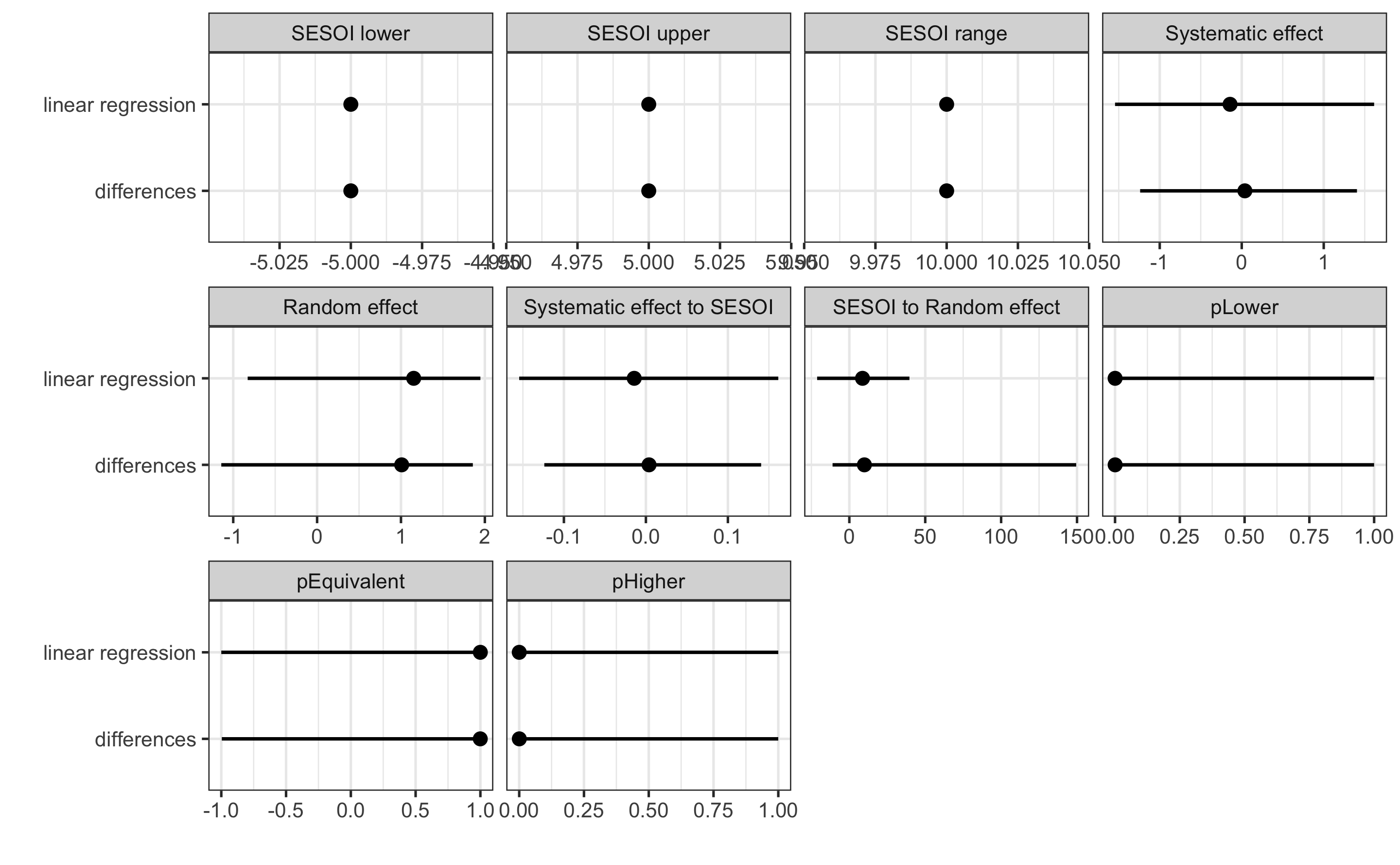
Which method should be used? For simple designs, these provide almost identical results. We could perform simulations as we have done in the Validity and Reliability chapter to see the behavior of the estimates, but I will leave that to you as an exercise. I would generally follow the advice by Frank Harrell and avoid the use of the change scores, particularly for more complex designs involving covariates and extra parameters of the treatment (i.e. when treatment is not only TRUE/FALSE but can have a continuous membership function, or some type of the loading parameter, like number of jumps performed and so forth).
16.4 Prediction perspective 1
Using simple linear regression function brings us to the prediction perspective of modeling the RCT data. Rather than estimating DGP parameters, we are interested in predicting individual responses on the unseen data. We can thus use bmbstats::cv_model function to estimate predictive performance of our simple linear regression model. One thing to keep in mind, is that now we are using SESOI to judge the residuals magnitudes, not observed scores (i.e. measured Post-test). Please note that I have used Group column to setup the CV strata - this results in same number of CV observations in each group.
model3 <- cv_model(
  Measured_score.Post ~ Measured_score.Pre + Group,
  RCT_data,
  SESOI_lower = -5,
  SESOI_upper = 5,
  control = model_control(
    seed = 1667,
    cv_folds = 3,
    cv_repeats = 10,
    cv_strata = factor(RCT_data$Group)
  )
)

model3
#> Training data consists of 3 predictors and 20 observations.
#> Cross-Validation of the model was performed using 10 repeats of 3 folds.
#>
#> Model performance:
#>
#>         metric      training training.pooled testing.pooled        mean         SD
#>            MBE  2.202681e-14    1.918475e-15    -0.04123424 -0.06466644 0.91228266
#>            MAE  1.176009e+00    1.125490e+00     1.47603175  1.47790175 0.33700044
#>           RMSE  1.473109e+00    1.403919e+00     1.82619034  1.79036050 0.37125297
#>           PPER  9.963039e-01    9.995798e-01     0.99312088  0.96151334 0.02661372
#>  SESOI to RMSE  6.788364e+00    7.122918e+00     5.47588047  5.82060839 1.20914378
#>      R-squared  9.235673e-01    9.305786e-01     0.88259682  0.86160357 0.10805679
#>         MinErr -3.138804e+00   -3.623411e+00    -5.03757174 -2.56189890 1.14780901
#>         MaxErr  2.600139e+00    2.890624e+00     3.53991399  2.08918814 0.96885433
#>      MaxAbsErr  3.138804e+00    3.623411e+00     5.03757174  3.08675364 0.76498989
#>         min       max
#>  -2.0716103 1.8762924
#>   0.8701076 2.0982105
#>   1.1312614 2.6810220
#>   0.8929713 0.9939017
#>   3.7299209 8.8396899
#>   0.5866306 0.9743506
#>  -5.0375717 0.3235147
#>  -0.4470821 3.5399140
#>   1.7111147 5.0375717
As can be seen from the performance results, we have pretty good prediction of the individual responses since our SESOI is pretty large and we do not have any treatment nor non-treatment effects.
bmbstats package comes with additional function bmbstats::RCT_predict that uses returned object by bmbstats::cv_model and analyze is from RCT perspective:
prediction_RCT <- RCT_predict(
  model3,
  new_data = RCT_data,
  outcome = "Measured_score.Post",
  group = "Group",
  treatment_label = "Treatment",
  control_label = "Control",
  subject_label = RCT_data$Athlete
)

prediction_RCT
#> Training data consists of 3 predictors and 20 observations.
#> Cross-Validation of the model was performed using 10 repeats of 3 folds.
#>
#> Model performance:
#>
#>         metric      training training.pooled testing.pooled        mean         SD
#>            MBE  2.202681e-14    1.918475e-15    -0.04123424 -0.06466644 0.91228266
#>            MAE  1.176009e+00    1.125490e+00     1.47603175  1.47790175 0.33700044
#>           RMSE  1.473109e+00    1.403919e+00     1.82619034  1.79036050 0.37125297
#>           PPER  9.963039e-01    9.995798e-01     0.99312088  0.96151334 0.02661372
#>  SESOI to RMSE  6.788364e+00    7.122918e+00     5.47588047  5.82060839 1.20914378
#>      R-squared  9.235673e-01    9.305786e-01     0.88259682  0.86160357 0.10805679
#>         MinErr -3.138804e+00   -3.623411e+00    -5.03757174 -2.56189890 1.14780901
#>         MaxErr  2.600139e+00    2.890624e+00     3.53991399  2.08918814 0.96885433
#>      MaxAbsErr  3.138804e+00    3.623411e+00     5.03757174  3.08675364 0.76498989
#>         min       max
#>  -2.0716103 1.8762924
#>   0.8701076 2.0982105
#>   1.1312614 2.6810220
#>   0.8929713 0.9939017
#>   3.7299209 8.8396899
#>   0.5866306 0.9743506
#>  -5.0375717 0.3235147
#>  -0.4470821 3.5399140
#>   1.7111147 5.0375717
#>
#> Individual model results:
#>
#>     subject     group observed predicted    residual  magnitude counterfactual      pITE
#>  Athlete 01 Treatment 53.06613  51.87749 -1.18864415 Equivalent       52.01990  0.142417
#>  Athlete 02   Control 41.74203  42.17581  0.43378581 Equivalent       42.03340 -0.142417
#>  Athlete 03 Treatment 51.26538  48.12658 -3.13880386 Equivalent       48.26899  0.142417
#>  Athlete 04   Control 44.89588  44.04977 -0.84610959 Equivalent       43.90736 -0.142417
#>  Athlete 05 Treatment 39.31947  41.54657  2.22709299 Equivalent       41.68898  0.142417
#>  Athlete 06   Control 41.15527  42.16271  1.00744225 Equivalent       42.02030 -0.142417
#>  Athlete 07 Treatment 40.80646  42.76857  1.96211098 Equivalent       42.91099  0.142417
#>  Athlete 08   Control 48.68788  48.15176 -0.53612109 Equivalent       48.00934 -0.142417
#>  Athlete 09 Treatment 33.26669  33.21228 -0.05441276 Equivalent       33.35469  0.142417
#>  Athlete 10   Control 45.90508  44.34223 -1.56285495 Equivalent       44.19981 -0.142417
#>  Athlete 11 Treatment 33.61544  34.37183  0.75639501 Equivalent       34.51425  0.142417
#>  Athlete 12   Control 43.34150  45.94164  2.60013908 Equivalent       45.79923 -0.142417
#>  Athlete 13 Treatment 40.88270  38.87404 -2.00866163 Equivalent       39.01645  0.142417
#>  Athlete 14   Control 50.96896  50.99231  0.02334441 Equivalent       50.84989 -0.142417
#>  Athlete 15 Treatment 42.08253  41.84993 -0.23260068 Equivalent       41.99235  0.142417
#>  Athlete 16   Control 49.26936  50.30751  1.03815067 Equivalent       50.16510 -0.142417
#>  Athlete 17 Treatment 40.00091  39.96681 -0.03410111 Equivalent       40.10923  0.142417
#>  Athlete 18   Control 41.32829  39.57284 -1.75545843 Equivalent       39.43042 -0.142417
#>  Athlete 19 Treatment 49.12101  50.83263  1.71162522 Equivalent       50.97505  0.142417
#>  Athlete 20   Control 43.96351  43.56119 -0.40231815 Equivalent       43.41878 -0.142417
#>  pITE_magnitude
#>      Equivalent
#>      Equivalent
#>      Equivalent
#>      Equivalent
#>      Equivalent
#>      Equivalent
#>      Equivalent
#>      Equivalent
#>      Equivalent
#>      Equivalent
#>      Equivalent
#>      Equivalent
#>      Equivalent
#>      Equivalent
#>      Equivalent
#>      Equivalent
#>      Equivalent
#>      Equivalent
#>      Equivalent
#>      Equivalent
#>
#> Summary of residuals per RCT group:
#>
#>      group         mean       SD
#>    Control 1.634246e-14 1.322097
#>  Treatment 2.771120e-14 1.753394
#>
#> Summary of counterfactual effects of RCT group:
#>
#>      group      pATE pVTE
#>  Treatment  0.142417    0
#>    Control -0.142417    0
#>     pooled  0.142417    0
#>
#> Treatment effect summary
#>
#> Average Treatment effect:  0.142417
#> Variable Treatment effect:  0
#> Random Treatment effect:  1.151716
The results of bmbstats::RCT_predict contain (1) model performance (also returned from bmbstats::cv_model), (2) individual model results (which contains individual model predictions, as well as counterfactual predictions assuming Group changes from Control to Treatment and vice versa), (3) residuals summary per group (these are our random effects), and (4) summary of counterfactual effects (please refer to Causal inference chapter for more information about these concepts). The extra details that bmbstats::RCT_predict adds on top of bmbstats::cv_model can be found in the prediction_RCT$extra.
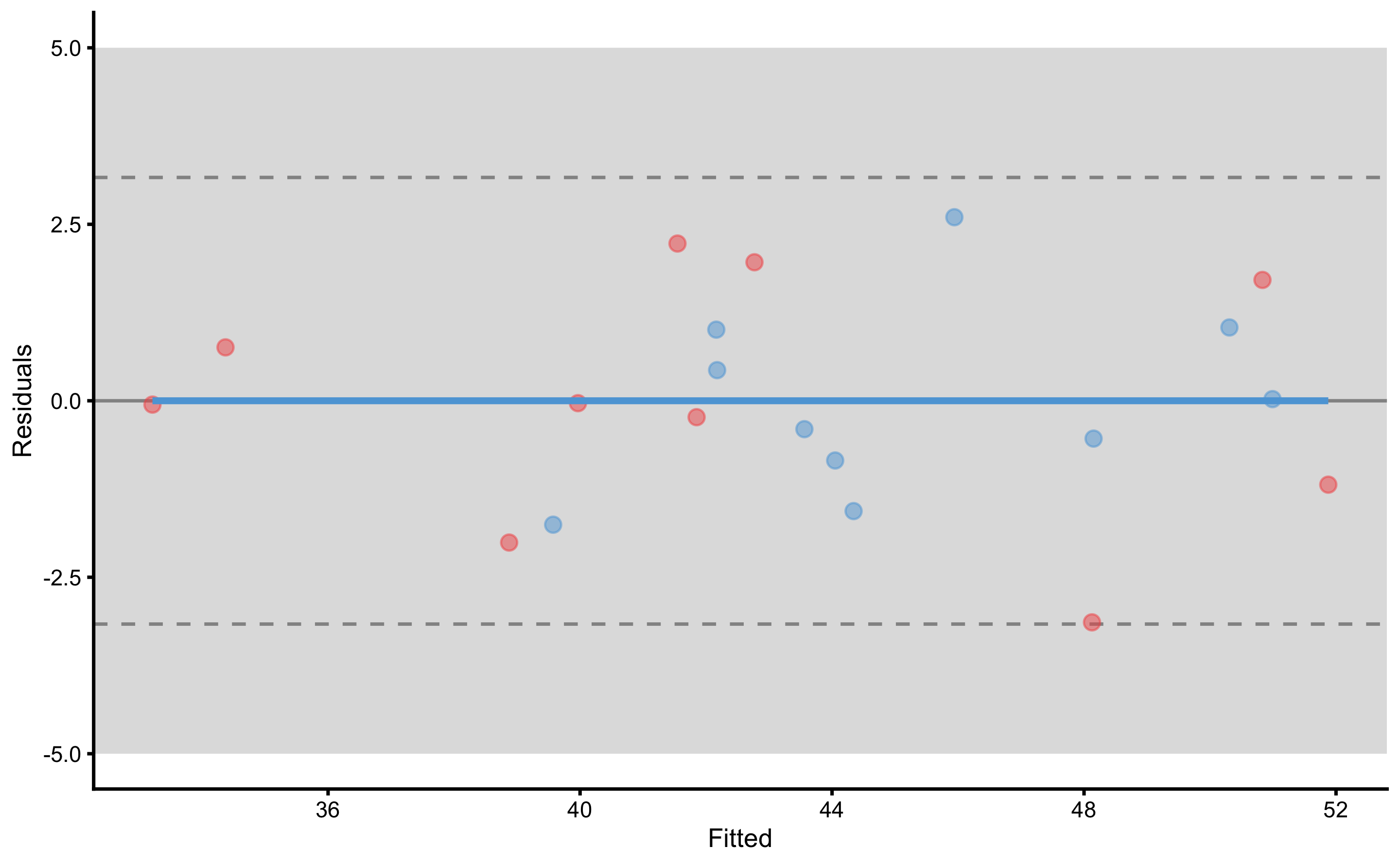
Now that we have the more info about the underlying RCT, we can do various plots. Let’s plot the residuals first:
To plot individual model predictions use the following:
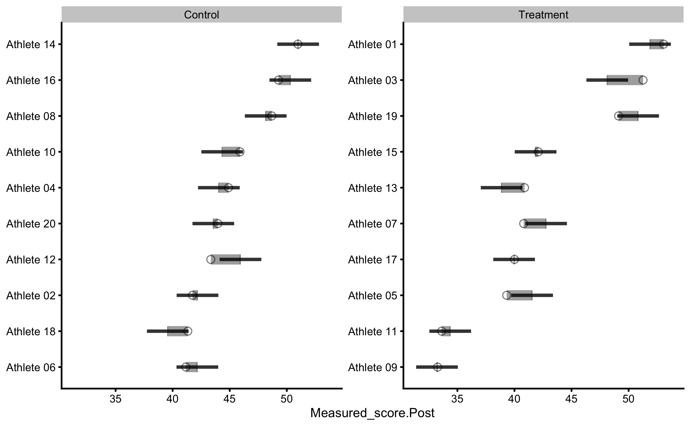
Circlets or dots represent observed (i.e. outcome or target variable), and vertical line represent model predictions. Residual between the two is color coded based on the provided SESOI threshold.
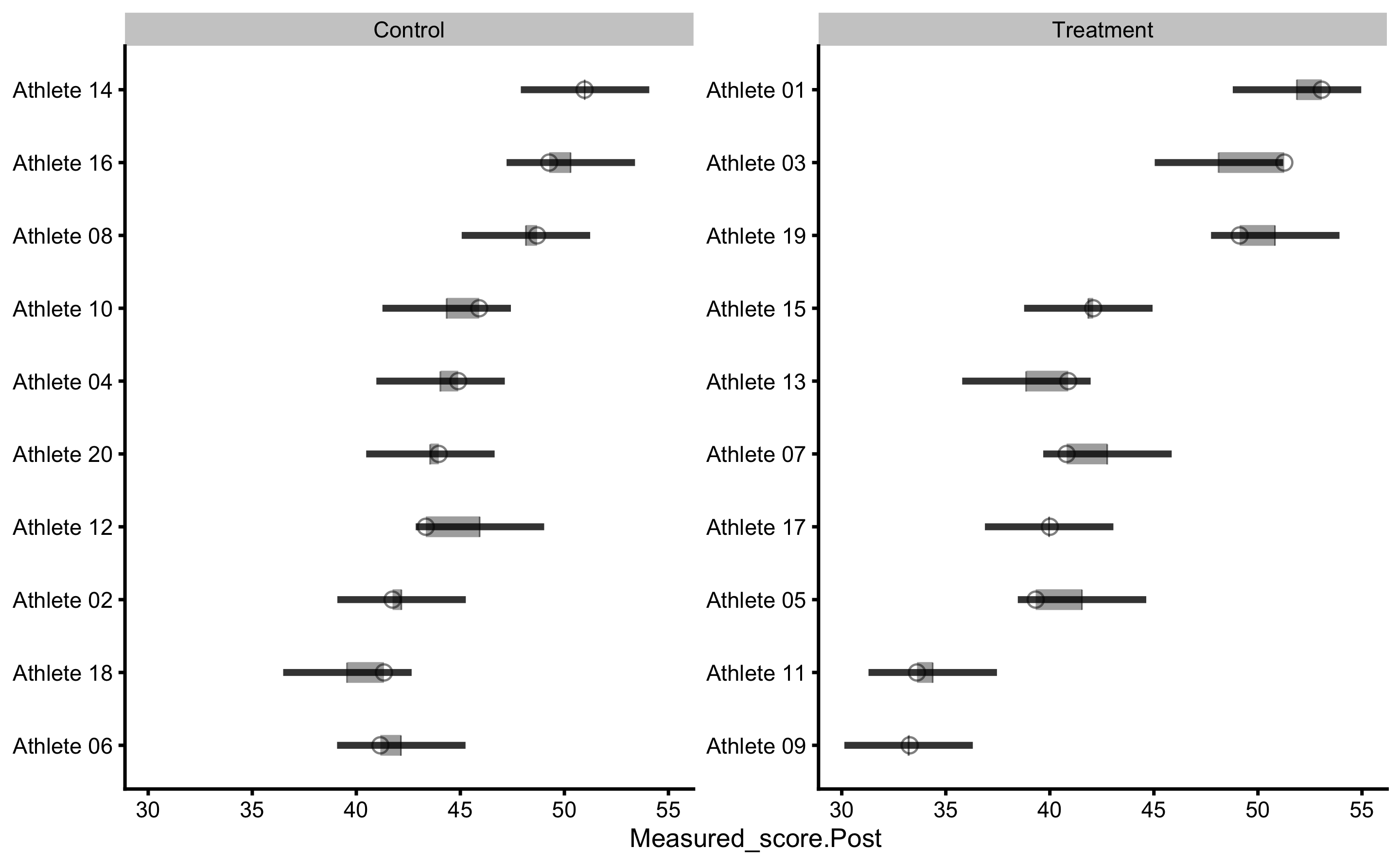
By default, prediction plot uses metric = "RMSE" and metric_cv = "testing.pooled" parameters to plot confidence intervals. We can use some other metric returned from bmbstats::cv_model. Let’s use MaxAbsErr (maximum absolute prediction error) from mean testing CV column:
To plot individual bias-variance error decomposition thorough testing CV folds use:
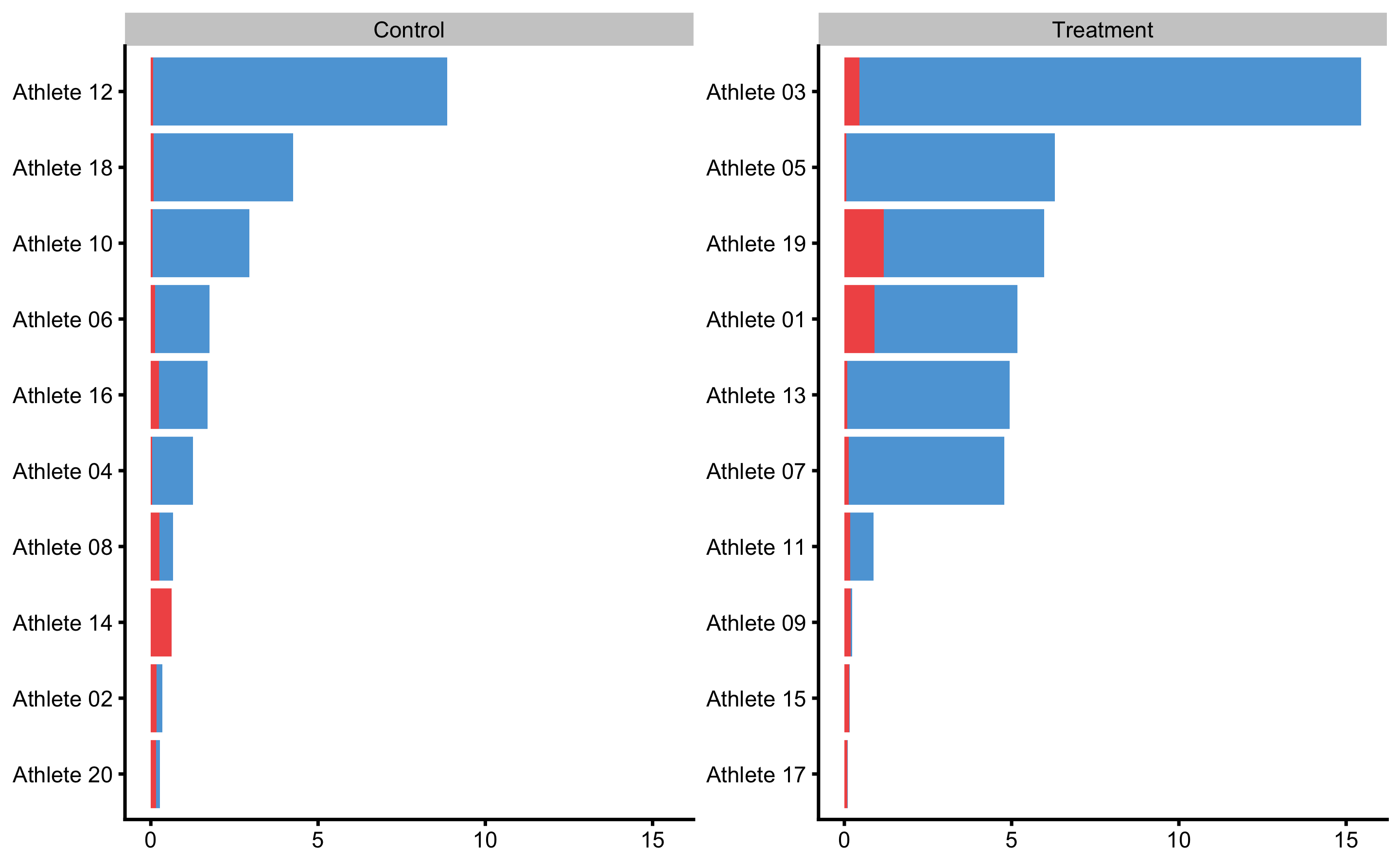
Here we can see which athletes are prediction outliers and generally present issues for the predictive model. Together with the individual predictions, we can use this plot and data to gain more info regarding individual reactions to intervention (i.e. who jumps out from the model prediction).
To gain understanding into counterfactual prediction, we could use PDP and ICE plots. The default variable to be used is the Group, which we can change later:
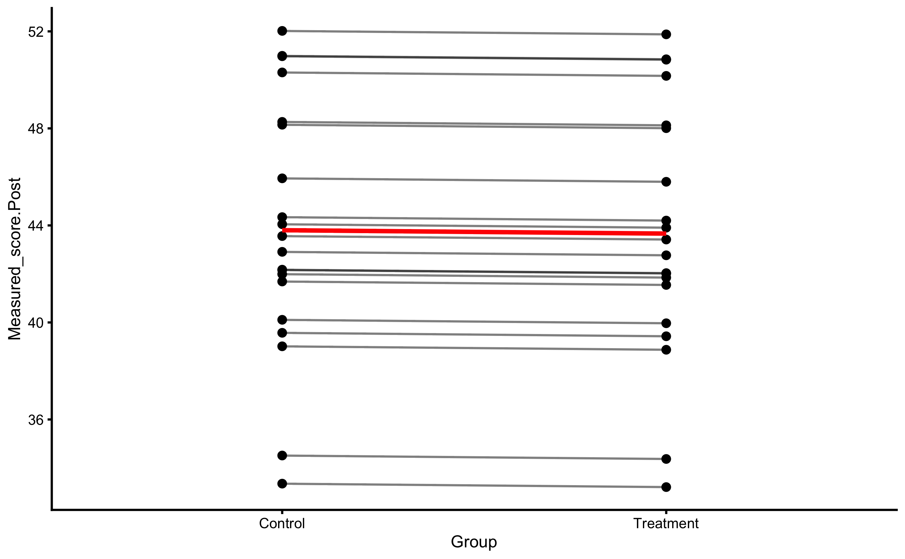
This plot gives us insights into model prediction for each athlete when the Group variable changes, while keeping all other variables the same. Since this is RCT, this plot can be given counterfactual interpretation. The PDP line (thick red line) represent the average of these individual prediction (ICE lines), and as can be seen, the counterfactual effects of changing group is zero (since the line is parallel) and thus represents expected or systematic effect of the treatment.
Let’s do that for out other variable in the model (with addition of the dashed identity line):
plot(prediction_RCT, "pdp+ice", predictor = "Measured_score.Pre") +
  geom_abline(slope = 1, linetype = "dashed")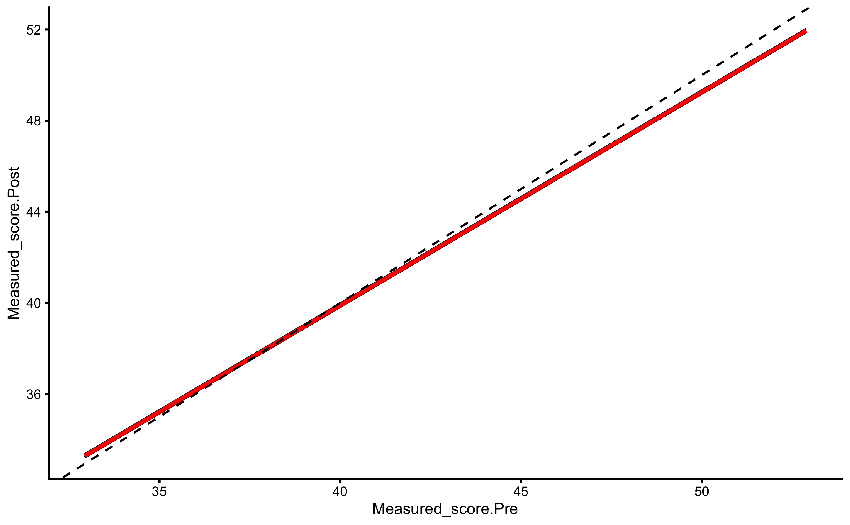
To plot these individual ICE line for each athlete we can use counterfactual plot:
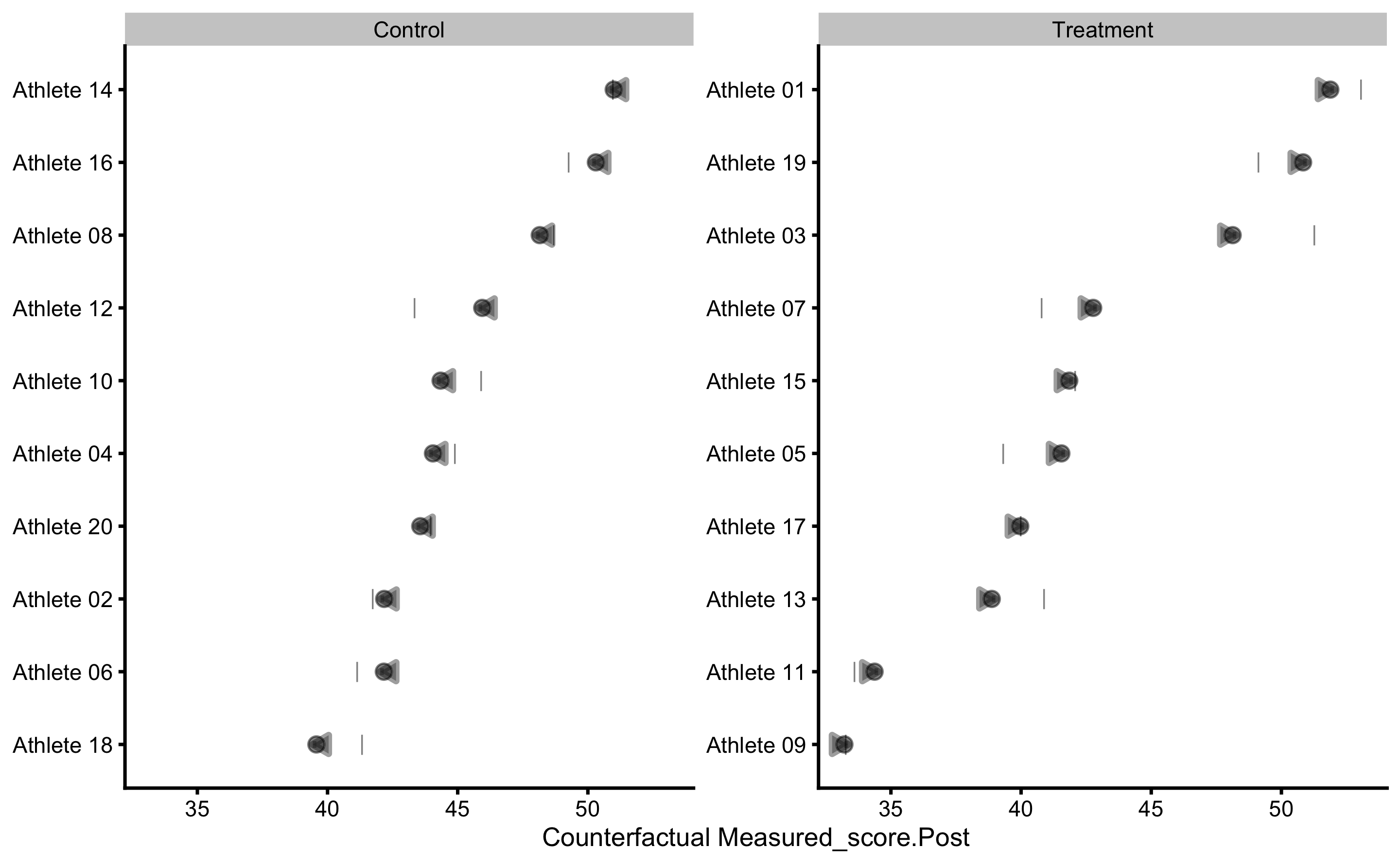
Since the systematic treatment effect is zero, these are very small. The mean of these individual counterfactual prediction effect is presented in the object printout in the last table as pATE (predicted average treatment effect) and SD of these effects as pVTE (predicted variable treatment effect). In this case, due simple model, the predicted treatment effects are the same, thus the pVTE is equal to zero.
Different way to plot these is to have trellis plot for each individual:
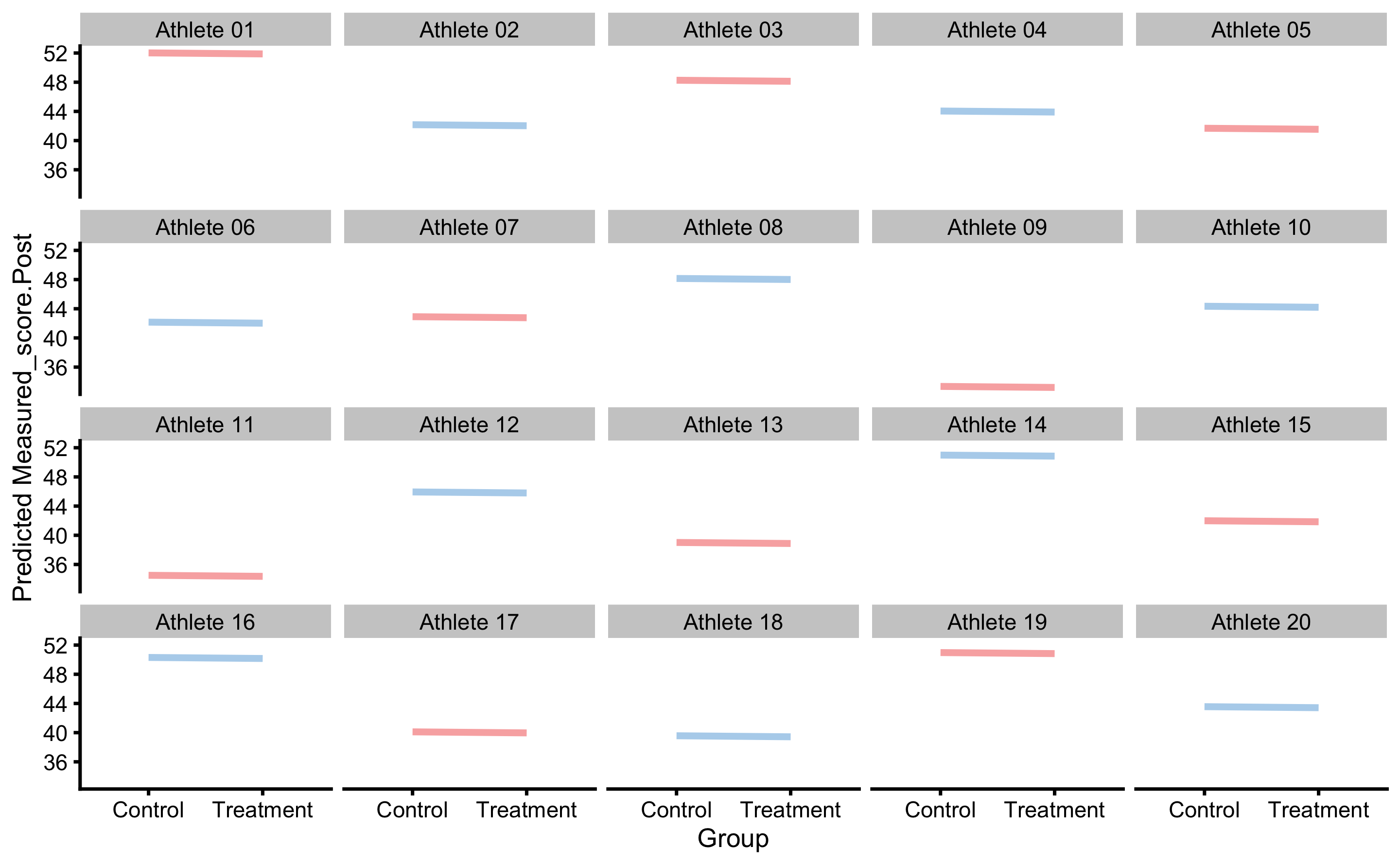
These plots represent strong tool for understanding predictive model performance for the RCT data and study designs.
16.5 Adding some effects
The previous example contained no treatment nor non-treatment effects, only biological variation and instrumentation noise. Let’s now consider different treatment - plyometric training that has systematic effect of 5cm (mean or expected change) and random effect of 5cm. But, since this study is done after the off-season, all athletes experienced systematic effect of 2.5cm increase and random effect of 1cm only by normal training. This represents non-treatment effect.
Biological variation (1.5cm) and instrumentation noise (0.5cm) are still involved in the measured scores.
This is the code to generate the data (i.e. DGP):
set.seed(16)

n_subjects <- 20

# These stay the same
instrumentation_noise <- 0.5
biological_variation <- 1.5

# -------------------------
# Treatment effect
treatment_systematic <- 5
treatment_random <- 5

# Non-treatment effect
non_treatment_systematic <- 2.5
non_treatment_random <- 1
#-------------------------

RCT_data <- tibble(
  Athlete = paste(
    "Athlete",
    str_pad(
      string = seq(1, n_subjects),
      width = 2,
      pad = "0"
    )
  ),
  Group = rep(c("Treatment", "Control"), length.out = n_subjects),

  # True score
  True_score.Pre = rnorm(n_subjects, 45, 5),

  # Treatment effect
  Treatment_effect = rnorm(
    n = n_subjects,
    mean = treatment_systematic,
    sd = treatment_random),

  Non_treatment_effect = rnorm(
    n = n_subjects,
    mean = non_treatment_systematic,
    sd = non_treatment_random),

  # Calculate the change in true score
  True_score.Change = if_else(
    Group == "Treatment",
    # Treatment group is a sum of treatment and non-treatment effects
    Treatment_effect + Non_treatment_effect,
    # While control group only get non-treatment effects
    Non_treatment_effect
  ),
  True_score.Post = True_score.Pre + True_score.Change,

  # Manifested score
  Manifested_score.Pre = True_score.Pre +
    rnorm(n_subjects, 0, biological_variation),

  Manifested_score.Post = True_score.Post +
    rnorm(n_subjects, 0, biological_variation),

  Manifested_score.Change = Manifested_score.Post -
    Manifested_score.Pre,

  # Measured score
  Measured_score.Pre = Manifested_score.Pre +
    rnorm(n_subjects, 0, instrumentation_noise),

  Measured_score.Post = Manifested_score.Post +
    rnorm(n_subjects, 0, instrumentation_noise),

  Measured_score.Change = Measured_score.Post -
    Measured_score.Pre
)

RCT_data$Group <- factor(RCT_data$Group)

head(RCT_data)
#> # A tibble: 6 x 13
#>   Athlete Group True_score.Pre Treatment_effect Non_treatment_e… True_score.Chan…
#>   <chr>   <fct>          <dbl>            <dbl>            <dbl>            <dbl>
#> 1 Athlet… Trea…           47.4           -3.24              1.17            -2.06
#> 2 Athlet… Cont…           44.4            3.43              4.57             4.57
#> 3 Athlet… Trea…           50.5            4.09              2.74             6.83
#> 4 Athlet… Cont…           37.8           12.4               2.15             2.15
#> 5 Athlet… Trea…           50.7            0.671             1.87             2.54
#> 6 Athlet… Cont…           42.7           12.6               2.78             2.78
#> # … with 7 more variables: True_score.Post <dbl>, Manifested_score.Pre <dbl>,
#> #   Manifested_score.Post <dbl>, Manifested_score.Change <dbl>, Measured_score.Pre <dbl>,
#> #   Measured_score.Post <dbl>, Measured_score.Change <dbl>
Let’s plot the data using Pre-test as predictor (x-axis) and Post-test as the outcome (y-axis). Please remember that this plot provide simple linear regression for each group independently. I will add identity line for easier comparison:
ggplot(
  RCT_data,
  aes(x = Measured_score.Pre, y = Measured_score.Post, color = Group, fill = Group)
) +
  theme_cowplot(8) +
  geom_abline(slope = 1, linetype = "dashed") +
  geom_smooth(method = "lm", se = TRUE, alpha = 0.2) +
  geom_point(alpha = 0.8) +
  scale_color_manual(values = c(Treatment = "#FAA43A", Control = "#5DA5DA")) +
  scale_fill_manual(values = c(Treatment = "#FAA43A", Control = "#5DA5DA"))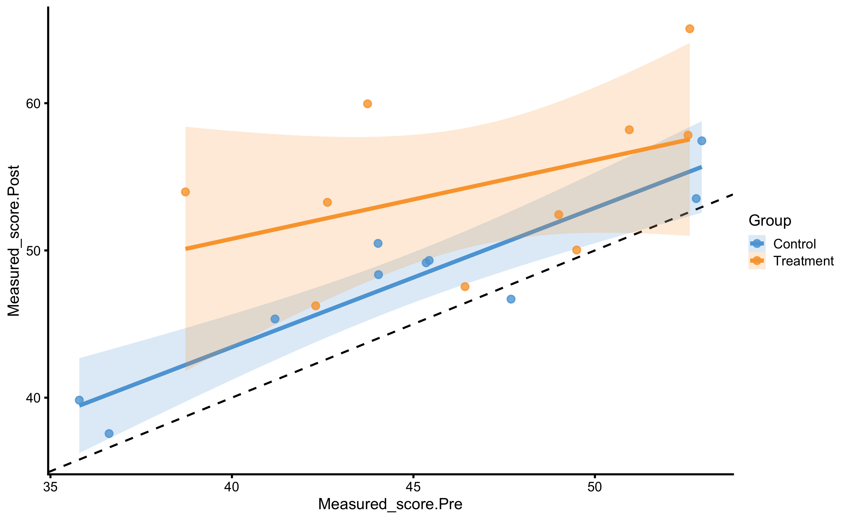
We can see that both Control and Treatment group demonstrated improvements since both lines are above the dashed identity line.
Using simple linear regression we get the following coefficients:
model4 <- lm(
  Measured_score.Post ~ Measured_score.Pre + Group,
  RCT_data
)

summary(model4)
#>
#> Call:
#> lm(formula = Measured_score.Post ~ Measured_score.Pre + Group,
#>     data = RCT_data)
#>
#> Residuals:
#>     Min      1Q  Median      3Q     Max
#> -6.5827 -3.5413  0.3856  2.3547  7.9219
#>
#> Coefficients:
#>                    Estimate Std. Error t value Pr(>|t|)
#> (Intercept)         13.1094     8.5876   1.527 0.145262
#> Measured_score.Pre   0.7774     0.1902   4.088 0.000767 ***
#> GroupTreatment       4.9265     1.9679   2.503 0.022784 *
#> ---
#> Signif. codes:  0 '***' 0.001 '**' 0.01 '*' 0.05 '.' 0.1 ' ' 1
#>
#> Residual standard error: 4.294 on 17 degrees of freedom
#> Multiple R-squared:  0.6289, Adjusted R-squared:  0.5853
#> F-statistic: 14.41 on 2 and 17 DF,  p-value: 0.000219
Now the simple linear regression estimated systematic treatment effect of 4.93cm, which is very close to our DGP systematic treatment effect of 5cm.
To estimate random treatment effect, we can use residuals SD for each group:
SD_summary <- RCT_data %>%
  mutate(.resid = residuals(model4)) %>%
  group_by(Group) %>%
  summarise(`Residual SD` = sd(.resid))

SD_summary
#> # A tibble: 2 x 2
#>   Group     `Residual SD`
#>   <fct>             <dbl>
#> 1 Control            2.41
#> 2 Treatment 5.39Using bmbstats::RCT_estimators_lm estimator function and bmbstats::RCT_analysis functions, let’s perform the analysis and generate 95% bootstrap confidence intervals:
regression_RCT <- bmbstats::RCT_analysis(
  data = RCT_data,
  group = "Group",
  treatment_label = "Treatment",
  control_label = "Control",
  pre_test = "Measured_score.Pre",
  post_test = "Measured_score.Post",
  SESOI_lower = -5,
  SESOI_upper = 5,
  estimator_function = bmbstats::RCT_estimators_lm,
  control = model_control(seed = 1667)
)
#> [1] "All values of t are equal to  5 \n Cannot calculate confidence intervals"
#> [1] "All values of t are equal to  10 \n Cannot calculate confidence intervals"


regression_RCT
#> Bootstrap with 2000 resamples and 95% bca confidence intervals.
#>
#>                   estimator       value         lower     upper
#>                 SESOI lower -5.00000000            NA        NA
#>                 SESOI upper  5.00000000            NA        NA
#>                 SESOI range 10.00000000            NA        NA
#>           Systematic effect  4.92654585   1.082956784 8.7715046
#>               Random effect  4.81651919   3.443713578 6.3838094
#>  Systematic effect to SESOI  0.49265458   0.108295678 0.8771505
#>      SESOI to Random effect  2.07618814 -21.118934945 2.9121218
#>                      pLower  0.02663292   0.001106225 0.2469677
#>                 pEquivalent  0.47937140   0.097391976 0.8405754
#>                     pHigher  0.49399568   0.117750794 0.8878213
Here is the estimators bootstrap distribution:
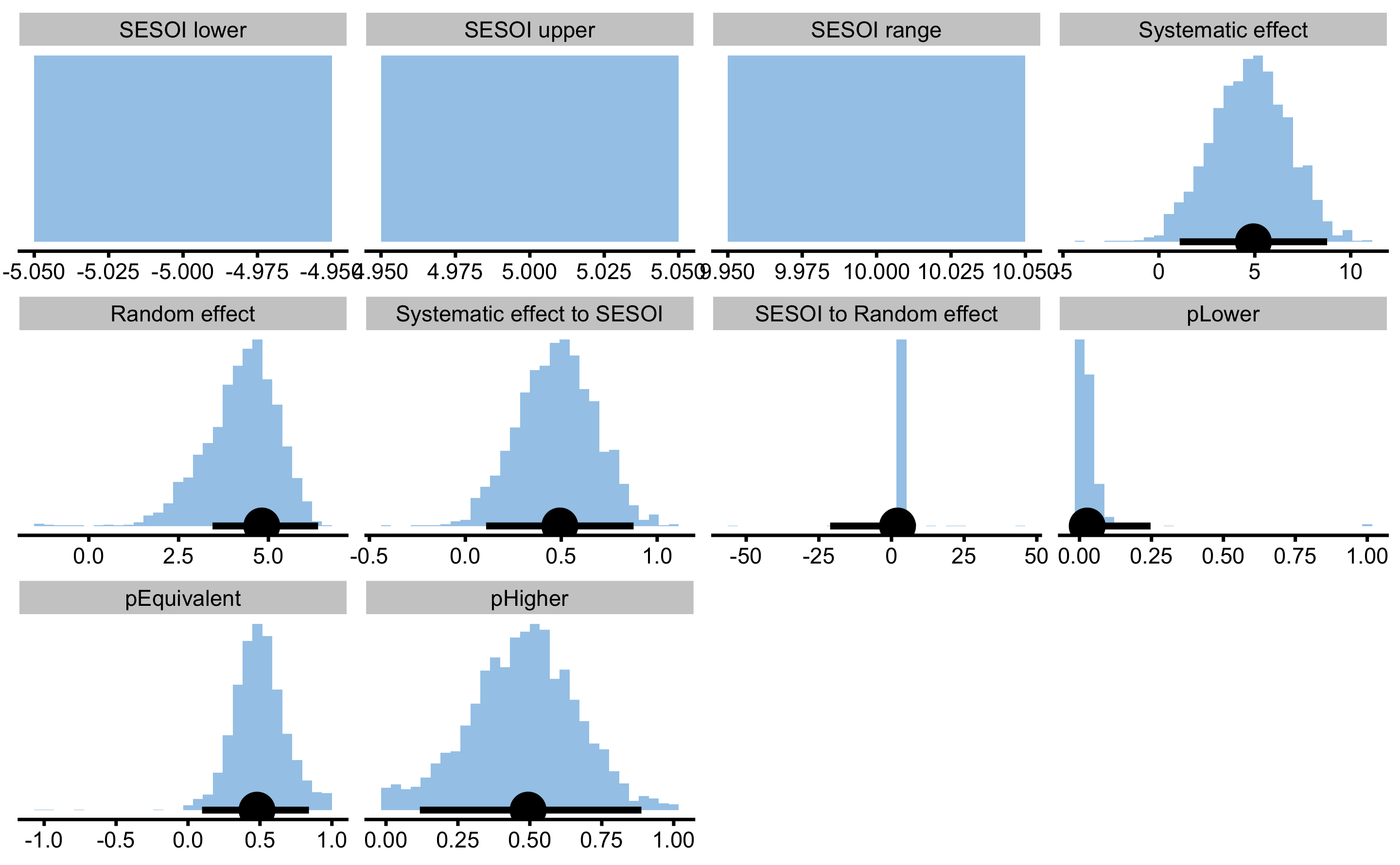
As can be seen from the results, both systematic and random components of the treatment effects were estimated correctly.
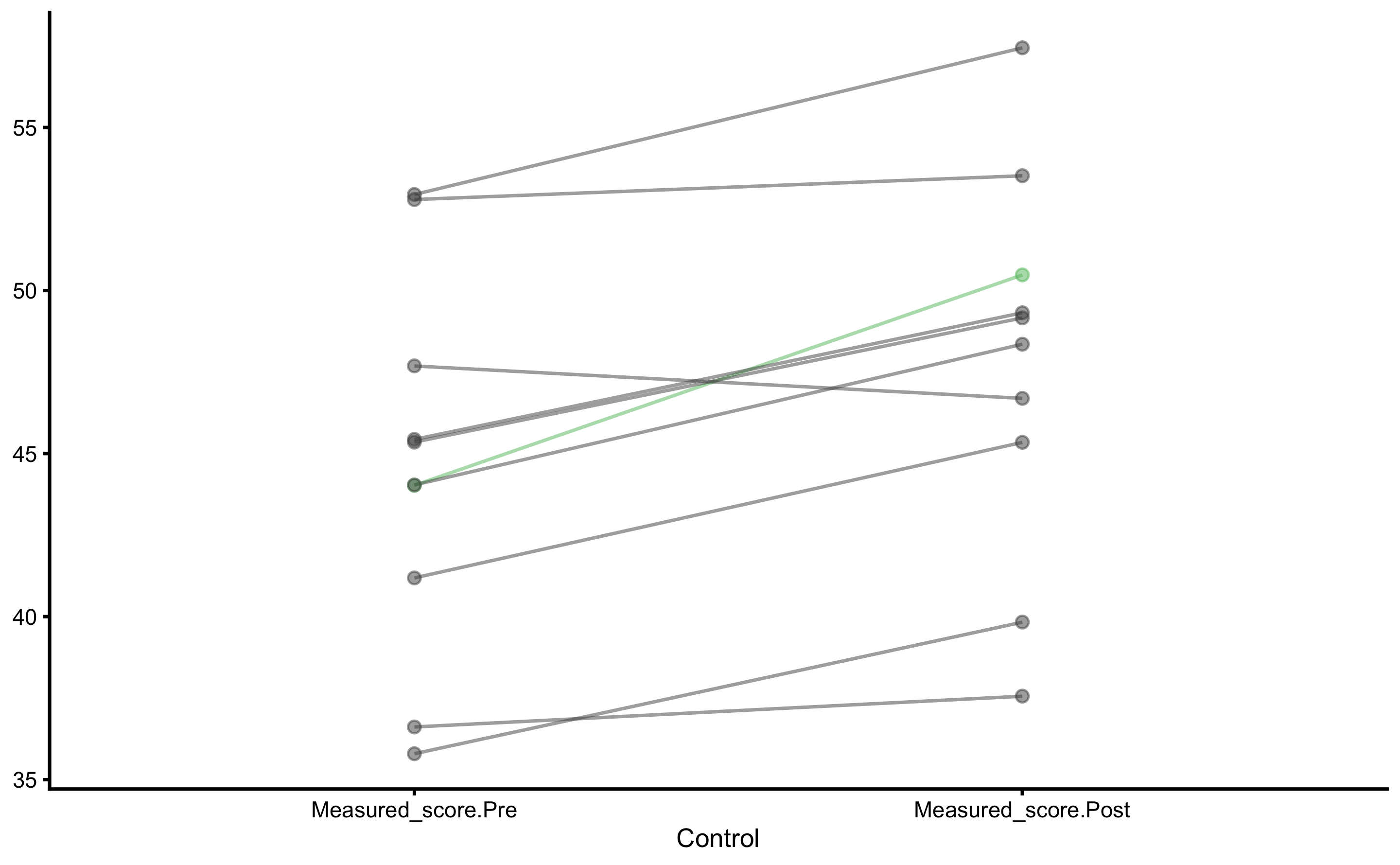
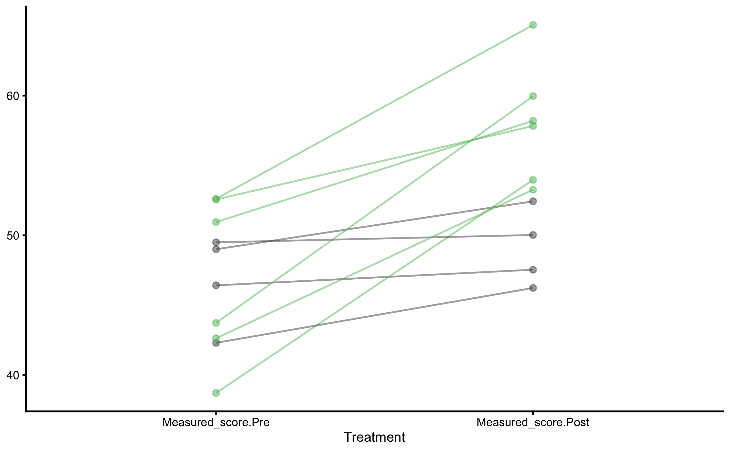
Let’s plot the Pre- and Post-Test results for each group (I will let you play and plot other figures as explained in the previous sections):
Let’s now plot individual treatment responses with uncertainty intervals:
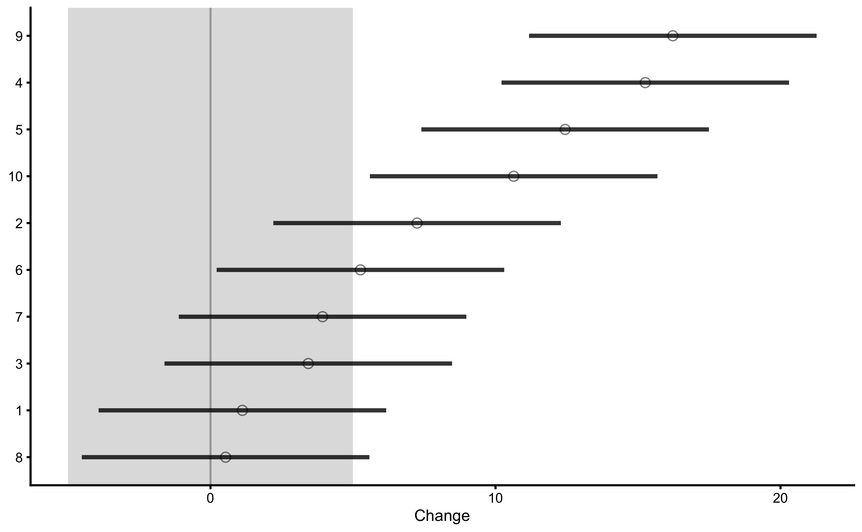
As explained previously, this type of analysis and plot, uses Control group change score as some type of a proxy to quantify the uncertainty around observed treatment group change scores. Please note that even though we have used linear regression approach to estimate treatment effects, the plots still rely on the change scores.
To check if this plot make sense, we can add the true treatment effects from the DGP using bmbstats::observations_MET function (we can also use bmbstats::observations_MBI function for plotting):
treatment_group <- filter(
  RCT_data,
  Group == "Treatment"
)

control_group <- filter(
  RCT_data,
  Group == "Control"
)

treatment_responses <- bmbstats::observations_MET(
  observations = treatment_group$Measured_score.Change,
  observations_label = treatment_group$Athlete,

  # Use control group change as measurement error
  measurement_error = sd(control_group$Measured_score.Change),

  # Degrees of freedom from the reliability study. Use `Inf` for normal distribution
  df = nrow(control_group) - 1,
  SESOI_lower = -5,
  SESOI_upper = 5,

  # Will not use Bonferroni adjustment here
  alpha = 0.05,
  # No adjustment in CIs for plotting
  confidence = 0.95
)

plot(
  treatment_responses,
  true_observations = treatment_group$True_score.Change,
  control = plot_control(points_size = 5)
) +
  xlim(-10, 28)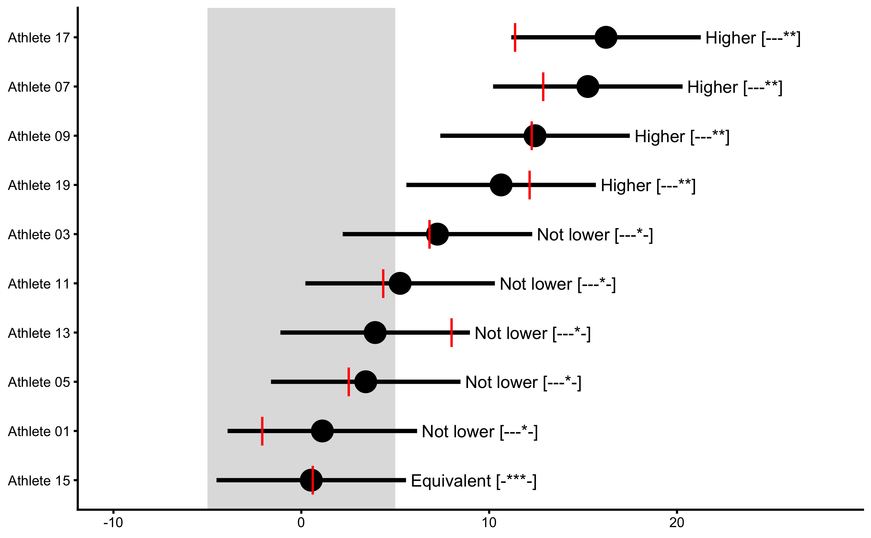
Adjusted treatment response would deduct mean change from the Control group and would show individual effect ONLY with treatment effect (without non-treatment effect). We can use our DGP generated data frame to generate that graph (or to recreate it) and plot true treatment effects:
treatment_responses <- bmbstats::observations_MET(

  # Adjustment
  observations = treatment_group$Measured_score.Change -
    mean(control_group$Measured_score.Change),

  observations_label = treatment_group$Athlete,

  # Use control group change as measurement error
  measurement_error = sd(control_group$Measured_score.Change),

  # Degrees of freedom from the reliability study. Use `Inf` for normal distribution
  df = nrow(control_group) - 1,
  SESOI_lower = -5,
  SESOI_upper = 5,

  # Will not use Bonferroni adjustment here
  alpha = 0.05,
  # No adjustment in CIs for plotting
  confidence = 0.95
)

plot(
  treatment_responses,
  # The true observation now is the DGP Treatment effect only
  true_observations = treatment_group$Treatment_effect,
  control = plot_control(points_size = 5)
) +
  xlim(-10, 28)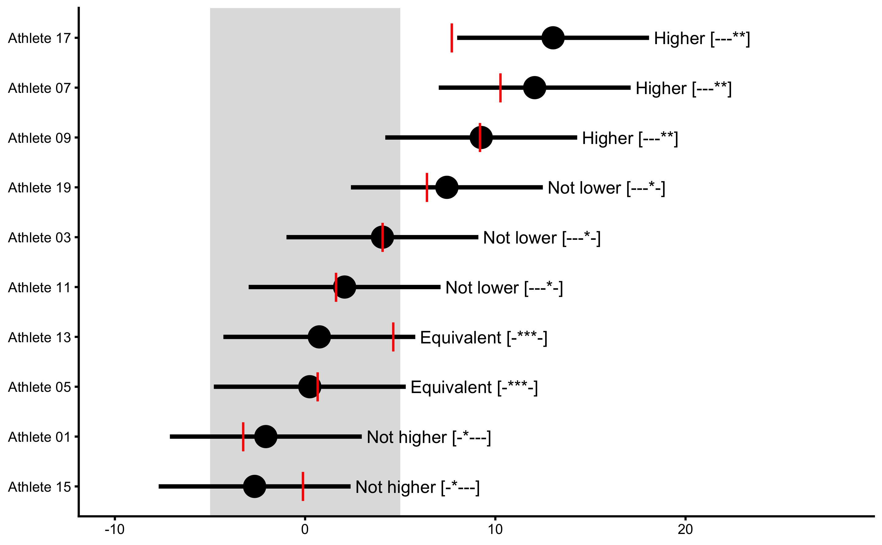
16.6 What goes inside the measurement error (or Control group change or residuals SD)?
As already explained, Control group serves as a counter-factual proxy of what would happen to the treatment group if not-receiving the treatment. SD of Control group change is used to represent an estimate of uncertainty around individual responses. In our RCT data, SD of the Control group measured change is equal to 2.23cm. This is equal to the root of squared sums of non-treatment random effect, biological variation and instrumentation noise. Since biological variation (BV) and instrumentation noise (IN) affects the change score twice (at Pre- and Post-test) we get the following (where NTRE is Non-treatment effect random error):
\[\begin{equation} SD_{control\;change} = \sqrt{2\times BV^2 + 2\times IN^2 + NTRE^2} \end{equation}\]
If we plug our DGP values, we get the following expected SD of the Control group change: 2.45cm. If there is no non-treatment random effect, then SD for the control group would only consist of measurement error.
This measurement error decomposition belongs to the method of differences, but the same error decomposition happens in the SD of the residuals with the linear regression approach.
To demonstrate this, consider random treatment effect estimated using the measured Pre-test and Post-test scores, versus using True scores.
model_true <- lm(
  True_score.Post ~ True_score.Pre + Group,
  RCT_data
)

summary(model_true)
#>
#> Call:
#> lm(formula = True_score.Post ~ True_score.Pre + Group, data = RCT_data)
#>
#> Residuals:
#>    Min     1Q Median     3Q    Max
#> -8.945 -1.128  0.299  1.822  6.053
#>
#> Coefficients:
#>                Estimate Std. Error t value Pr(>|t|)
#> (Intercept)     13.7253     8.2176   1.670 0.113184
#> True_score.Pre   0.7578     0.1801   4.208 0.000591 ***
#> GroupTreatment   4.6334     1.7272   2.683 0.015736 *
#> ---
#> Signif. codes:  0 '***' 0.001 '**' 0.01 '*' 0.05 '.' 0.1 ' ' 1
#>
#> Residual standard error: 3.764 on 17 degrees of freedom
#> Multiple R-squared:  0.6497, Adjusted R-squared:  0.6085
#> F-statistic: 15.76 on 2 and 17 DF,  p-value: 0.0001342
The model with measured scores is the model we have used so far (model4), but I am repeating it here for the sake of easier comprehension:
model_measured <- lm(
  Measured_score.Post ~ Measured_score.Pre + Group,
  RCT_data
)

summary(model_measured)
#>
#> Call:
#> lm(formula = Measured_score.Post ~ Measured_score.Pre + Group,
#>     data = RCT_data)
#>
#> Residuals:
#>     Min      1Q  Median      3Q     Max
#> -6.5827 -3.5413  0.3856  2.3547  7.9219
#>
#> Coefficients:
#>                    Estimate Std. Error t value Pr(>|t|)
#> (Intercept)         13.1094     8.5876   1.527 0.145262
#> Measured_score.Pre   0.7774     0.1902   4.088 0.000767 ***
#> GroupTreatment       4.9265     1.9679   2.503 0.022784 *
#> ---
#> Signif. codes:  0 '***' 0.001 '**' 0.01 '*' 0.05 '.' 0.1 ' ' 1
#>
#> Residual standard error: 4.294 on 17 degrees of freedom
#> Multiple R-squared:  0.6289, Adjusted R-squared:  0.5853
#> F-statistic: 14.41 on 2 and 17 DF,  p-value: 0.000219
Estimate random treatment effect for each model are the following, we can use residuals SD for each group:
SD_summary_true <- RCT_data %>%
  mutate(.resid = residuals(model_true)) %>%
  group_by(Group) %>%
  summarise(`Residual SD` = sd(.resid))

SD_summary_true
#> # A tibble: 2 x 2
#>   Group     `Residual SD`
#>   <fct>             <dbl>
#> 1 Control            1.47
#> 2 Treatment          4.96
The SD of the Control group residuals using the True scores should only involve random non-treatment effect, which is in our case equal to 1cm, and SD of the Treatment group residuals should be 5cm.
Let’s see whats the case with the model that uses Measured scores:
SD_summary_measured <- RCT_data %>%
  mutate(.resid = residuals(model_measured)) %>%
  group_by(Group) %>%
  summarise(`Residual SD` = sd(.resid))


SD_summary_measured
#> # A tibble: 2 x 2
#>   Group     `Residual SD`
#>   <fct>             <dbl>
#> 1 Control            2.41
#> 2 Treatment          5.39
The SD of the Control group residuals using the measured scores should now involve random non-treatment effect (1cm), 2 x biological variation (1.5cm) and 2 x instrumentation noise (0.5cm), which is around \(\sqrt{1^2 + 2 \times 1.5^2 + 2 \times 0.5^2}\), or 2.45cm.
The SD of the Treatment group residuals using the measured scores should now involve random non-treatment effect (1cm), 2 x biological variation (1.5cm), 2 x instrumentation noise (0.5cm), and additional random treatment effect (5cm) which is around \(\sqrt{1^2 + 2 \times 1.5^2 + 2 \times 0.5^2 + 5^2}\), or 5.57cm.
Estimated random treatment effects:
sqrt(SD_summary_measured$`Residual SD`[2]^2 - SD_summary_measured$`Residual SD`[1]^2)
#> [1] 4.816519
As can be seen, these are exactly the same. So, using measures scores and SD of control group change or residuals can recover true random treatment effect value.
16.7 Prediction perspective 2
Let’s see what happens when we run this RCT through predictive model.
model5 <- cv_model(
  Measured_score.Post ~ Measured_score.Pre + Group,
  RCT_data,
  SESOI_lower = -5,
  SESOI_upper = 5,
  control = model_control(
    seed = 1667,
    cv_folds = 3,
    cv_repeats = 10,
    cv_strata = factor(RCT_data$Group)
  )
)

prediction_RCT <- RCT_predict(
  model5,
  new_data = RCT_data,
  outcome = "Measured_score.Post",
  group = "Group",
  treatment_label = "Treatment",
  control_label = "Control",
  subject_label = RCT_data$Athlete
)

prediction_RCT
#> Training data consists of 3 predictors and 20 observations.
#> Cross-Validation of the model was performed using 10 repeats of 3 folds.
#>
#> Model performance:
#>
#>         metric      training training.pooled testing.pooled        mean         SD
#>            MBE -9.947541e-15    3.055367e-15     -0.1404122 -0.02732047 2.12193361
#>            MAE  3.175698e+00    3.037705e+00      3.8691755  3.90512133 0.93683875
#>           RMSE  3.959134e+00    3.786361e+00      4.7871794  4.73835660 0.85876892
#>           PPER  7.666283e-01    8.120334e-01      0.7012521  0.63888951 0.07928795
#>  SESOI to RMSE  2.525805e+00    2.641058e+00      2.0889127  2.17362777 0.37022957
#>      R-squared  6.289308e-01    6.606104e-01      0.4579491  0.21880124 0.64551950
#>         MinErr -7.921899e+00   -1.032365e+01    -10.0942651 -6.76317807 2.33015461
#>         MaxErr  6.582672e+00    8.806128e+00      9.2485263  6.05923474 2.11053360
#>      MaxAbsErr  7.921899e+00    1.032365e+01     10.0942651  8.02937811 1.17919840
#>          min        max
#>   -3.5145897  3.3371789
#>    2.6186933  6.8884587
#>    3.4284211  7.2937938
#>    0.4413183  0.7862394
#>    1.3710286  2.9167945
#>   -1.5780914  0.7986431
#>  -10.0942651 -2.7453015
#>    0.1401500  9.2485263
#>    5.5787979 10.0942651
#>
#> Individual model results:
#>
#>     subject     group observed predicted   residual  magnitude counterfactual      pITE
#>  Athlete 01 Treatment 47.54084  54.12352  6.5826720     Higher       49.19697 -4.926546
#>  Athlete 02   Control 50.47892  47.33454 -3.1443811 Equivalent       52.26108  4.926546
#>  Athlete 03 Treatment 58.19673  57.64224 -0.5544865 Equivalent       52.71569 -4.926546
#>  Athlete 04   Control 39.83268  40.93613  1.1034457 Equivalent       45.86267  4.926546
#>  Athlete 05 Treatment 52.43478  56.13132  3.6965427 Equivalent       51.20477 -4.926546
#>  Athlete 06   Control 45.34422  45.12752 -0.2166979 Equivalent       50.05407  4.926546
#>  Athlete 07 Treatment 53.97310  48.13585 -5.8372501      Lower       43.20931 -4.926546
#>  Athlete 08   Control 48.35425  47.34404 -1.0102111 Equivalent       52.27059  4.926546
#>  Athlete 09 Treatment 65.05732  58.93766 -6.1196617      Lower       54.01111 -4.926546
#>  Athlete 10   Control 46.69332  50.18284  3.4895230 Equivalent       55.10938  4.926546
#>  Athlete 11 Treatment 57.82698  58.90031  1.0733333 Equivalent       53.97377 -4.926546
#>  Athlete 12   Control 49.16140  48.36452 -0.7968803 Equivalent       53.29107  4.926546
#>  Athlete 13 Treatment 46.24005  50.92561  4.6855567 Equivalent       45.99907 -4.926546
#>  Athlete 14   Control 57.44395  54.26840 -3.1755549 Equivalent       59.19494  4.926546
#>  Athlete 15 Treatment 50.02857  56.51530  6.4867253     Higher       51.58875 -4.926546
#>  Athlete 16   Control 37.56101  41.57384  4.0128333 Equivalent       46.50039  4.926546
#>  Athlete 17 Treatment 59.95868  52.03678 -7.9218991      Lower       47.11023 -4.926546
#>  Athlete 18   Control 49.31810  48.42968 -0.8884198 Equivalent       53.35623  4.926546
#>  Athlete 19 Treatment 53.26809  51.17656 -2.0915325 Equivalent       46.25001 -4.926546
#>  Athlete 20   Control 53.52199  54.14833  0.6263431 Equivalent       59.07488  4.926546
#>  pITE_magnitude
#>      Equivalent
#>      Equivalent
#>      Equivalent
#>      Equivalent
#>      Equivalent
#>      Equivalent
#>      Equivalent
#>      Equivalent
#>      Equivalent
#>      Equivalent
#>      Equivalent
#>      Equivalent
#>      Equivalent
#>      Equivalent
#>      Equivalent
#>      Equivalent
#>      Equivalent
#>      Equivalent
#>      Equivalent
#>      Equivalent
#>
#> Summary of residuals per RCT group:
#>
#>      group          mean       SD
#>    Control -9.237121e-15 2.411836
#>  Treatment -1.065814e-14 5.386633
#>
#> Summary of counterfactual effects of RCT group:
#>
#>      group      pATE pVTE
#>  Treatment -4.926546    0
#>    Control  4.926546    0
#>     pooled  4.926546    0
#>
#> Treatment effect summary
#>
#> Average Treatment effect:  4.926546
#> Variable Treatment effect:  0
#> Random Treatment effect:  4.816519
The prediction performance in this case is much worse (compared to previous RCT example), since now there are systematic and random treatment and non-treatment effects. Although we can explain the RCT components, we cannot use it to predict individual responses.
Let’s check the individual predictions:
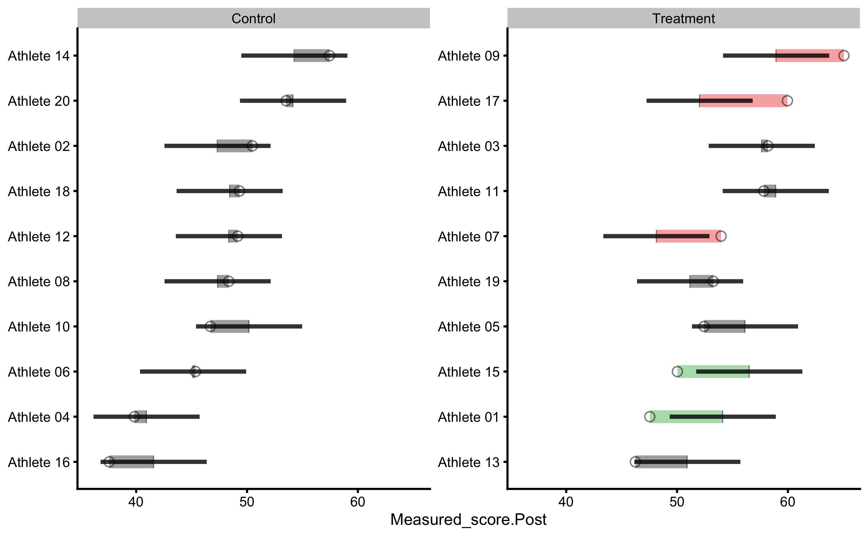
We can now see that certain residuals are larger than SESOI (indicated by green or red color on the figure).
Here is the PDP+ICE plot:
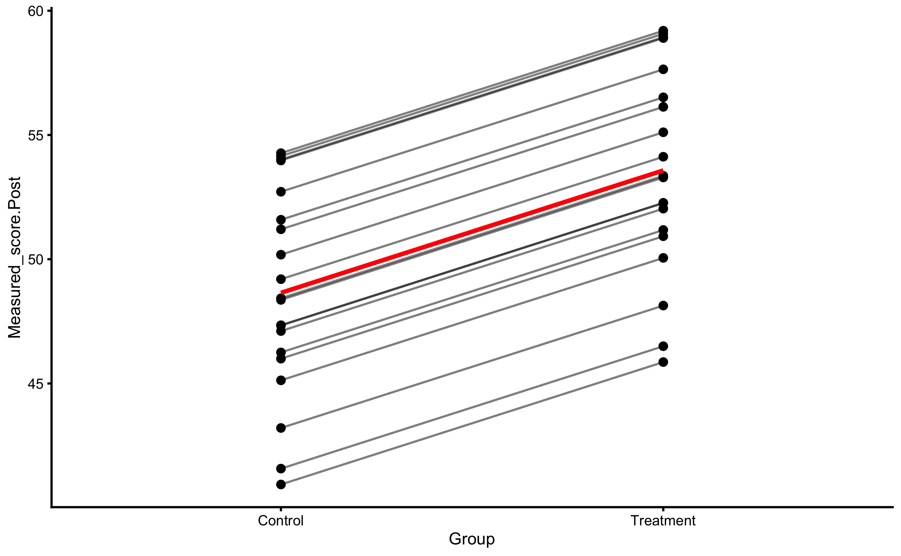
Parallel lines indicate that we predict that each individual will have same treatment effect (indicated by pVTE as well as with the arrows of same length in the counterfactual plot that follows). If we plot PDP+ICE for the measured Pre-test, we will get the following figure:
plot(prediction_RCT, "pdp+ice", predictor = "Measured_score.Pre") +
  geom_abline(slope = 1, linetype = "dashed")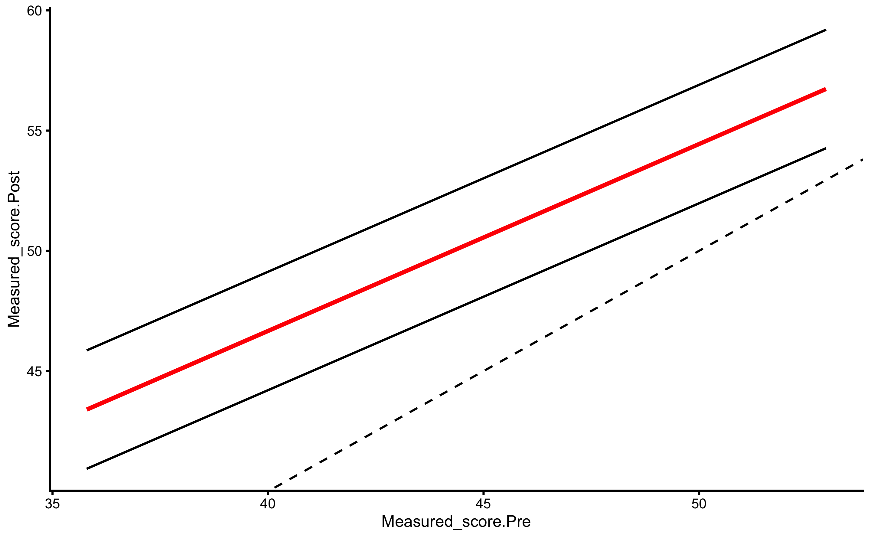
Two thin lines indicate two groups and the gap between them represents the systematic treatment effect.
Estimating individual counterfactual effects when switching group:
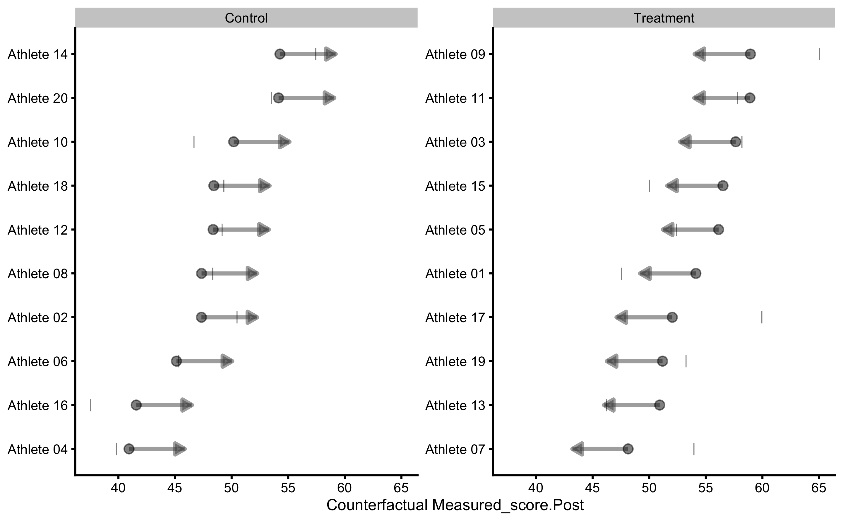
As can be seen, counterfactual plot depicts same treatment effect for every individual.
16.8 Making it more complex by adding covariate
To make this more complex, let’s assume that besides randomizing athletes to Treatment and Control group, we have also measured their lower body strength using relative back squat 1RM. This variable represents our covariate, and we can expect (i.e. we hypothesize) that individuals with higher relative strength will manifest bigger improvements from the plyometric intervention.
The following code represented DGP, where the effects of the training intervention depend on the 1RM squat (i.e. the higher the relative squat, the higher the training intervention). But on top of that, we are going to reduce the improvement based on the initial jump height (i.e. the higher someone jumps, the less improvement over time). It is assumed that squat 1RM and Pre-training jump height are unrelated (independent). Random components of the treatment and non-treatment effects are zero, and the only variance in the measured scores is due to biological noise and instrumentation error.
set.seed(16)

n_subjects <- 20

# These stay the same
instrumentation_noise <- 0.5
biological_variation <- 1.5

# -------------------------
# These are not used in this DGP
# Treatment effect
treatment_systematic <- 0
treatment_random <- 0

# Non-treatment effect
non_treatment_systematic <- 0
non_treatment_random <- 0
#-------------------------

RCT_data <- tibble(
  Athlete = paste(
    "Athlete",
    str_pad(
      string = seq(1, n_subjects),
      width = 2,
      pad = "0"
    )
  ),
  Group = rep(c("Treatment", "Control"), length.out = n_subjects),

  # Strength covariate
  Squat_1RM_relative = rnorm(n_subjects, 1, 0.4),
  # True score
  True_score.Pre = rnorm(n_subjects, 45, 5),

  # Treatment effect
  Treatment_effect = (10 - 0.002 * True_score.Pre^2 + 1) * Squat_1RM_relative,
  Non_treatment_effect = 15 - 0.005 * True_score.Pre^2,

  # Calculate the change in true score
  True_score.Change = if_else(
    Group == "Treatment",
    # Treatment group is a sum of treatment and non-treatment effects
    Treatment_effect + Non_treatment_effect,
    # While control group only get non-treatment effects
    Non_treatment_effect
  ),

  True_score.Post = True_score.Pre + True_score.Change,

  # Manifested score
  Manifested_score.Pre = True_score.Pre + rnorm(n_subjects, 0, biological_variation),
  Manifested_score.Post = True_score.Post + rnorm(n_subjects, 0, biological_variation),
  Manifested_score.Change = Manifested_score.Post - Manifested_score.Pre,

  # Measured score
  Measured_score.Pre = Manifested_score.Pre + rnorm(n_subjects, 0, instrumentation_noise),
  Measured_score.Post = Manifested_score.Post + rnorm(n_subjects, 0, instrumentation_noise),
  Measured_score.Change = Measured_score.Post - Measured_score.Pre
)

RCT_data$Group <- factor(RCT_data$Group)

head(RCT_data)
#> # A tibble: 6 x 14
#>   Athlete Group Squat_1RM_relat… True_score.Pre Treatment_effect Non_treatment_e…
#>   <chr>   <fct>            <dbl>          <dbl>            <dbl>            <dbl>
#> 1 Athlet… Trea…            1.19            36.8             9.88             8.24
#> 2 Athlet… Cont…            0.950           43.4             6.87             5.57
#> 3 Athlet… Trea…            1.44            44.1            10.2              5.28
#> 4 Athlet… Cont…            0.422           52.4             2.33             1.30
#> 5 Athlet… Trea…            1.46            40.7            11.2              6.73
#> 6 Athlet… Cont…            0.813           52.6             4.44             1.15
#> # … with 8 more variables: True_score.Change <dbl>, True_score.Post <dbl>,
#> #   Manifested_score.Pre <dbl>, Manifested_score.Post <dbl>,
#> #   Manifested_score.Change <dbl>, Measured_score.Pre <dbl>, Measured_score.Post <dbl>,
#> #   Measured_score.Change <dbl>
Let’s plot before we jump into the analysis. In the next plot we will depict measured Post-test (y-axis) and measured Pre-test (x-axis) per group.
ggplot(
  RCT_data,
  aes(x = Measured_score.Pre, y = Measured_score.Post, color = Group, fill = Group)
) +
  theme_cowplot(8) +
  geom_abline(slope = 1, linetype = "dashed") +
  geom_smooth(method = "lm", se = TRUE, alpha = 0.2) +
  geom_point(alpha = 0.8) +
  scale_color_manual(values = c(Treatment = "#FAA43A", Control = "#5DA5DA")) +
  scale_fill_manual(values = c(Treatment = "#FAA43A", Control = "#5DA5DA"))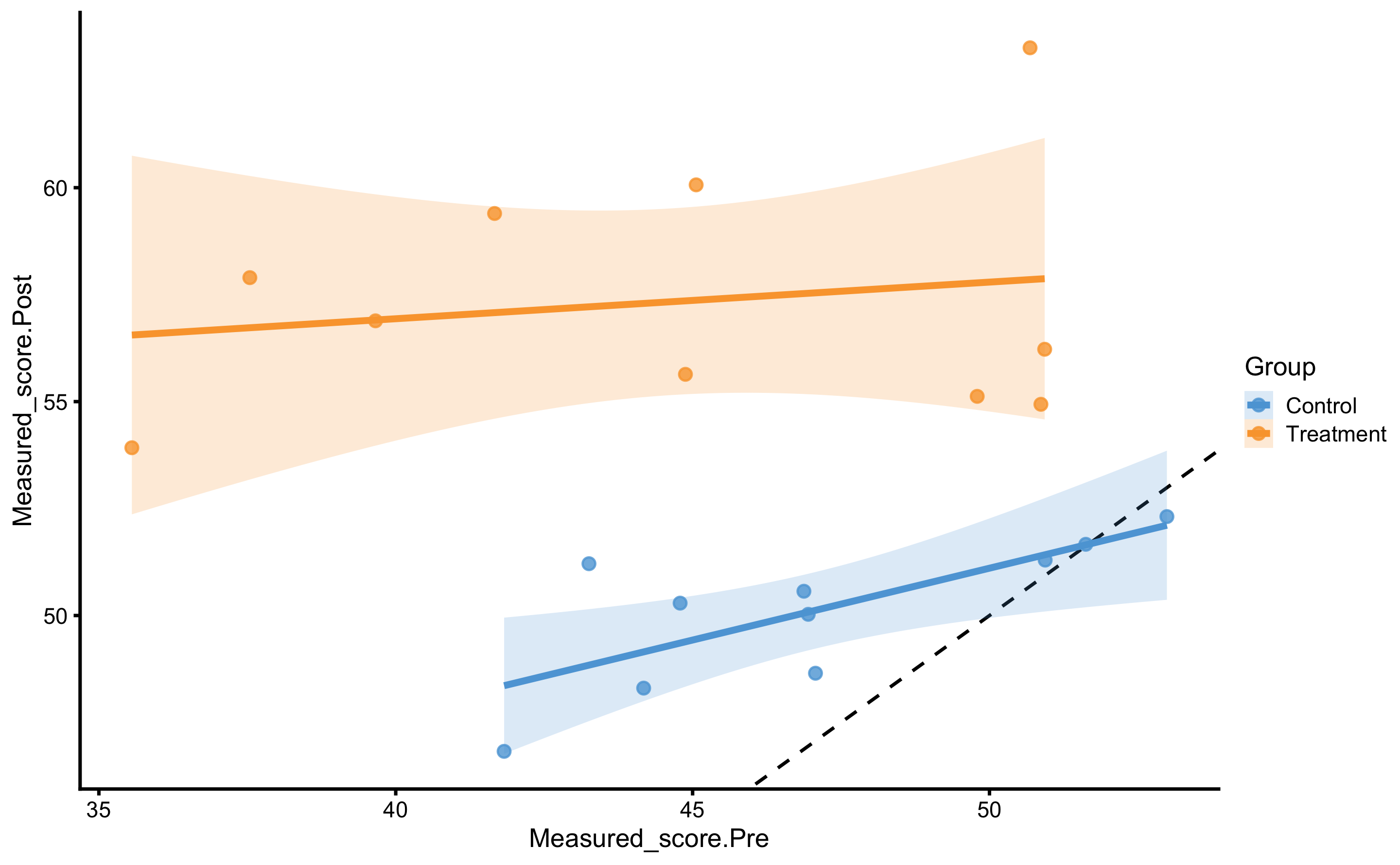
Might be also usable to plot the change score:
ggplot(
  RCT_data,
  aes(x = Measured_score.Pre, y = Measured_score.Change, color = Group, fill = Group)
) +
  theme_cowplot(8) +
  geom_smooth(method = "lm", se = TRUE, alpha = 0.2) +
  geom_hline(yintercept = 0, linetype = "dashed", alpha = 0.5) +
  geom_point(alpha = 0.8) +
  scale_color_manual(values = c(Treatment = "#FAA43A", Control = "#5DA5DA")) +
  scale_fill_manual(values = c(Treatment = "#FAA43A", Control = "#5DA5DA"))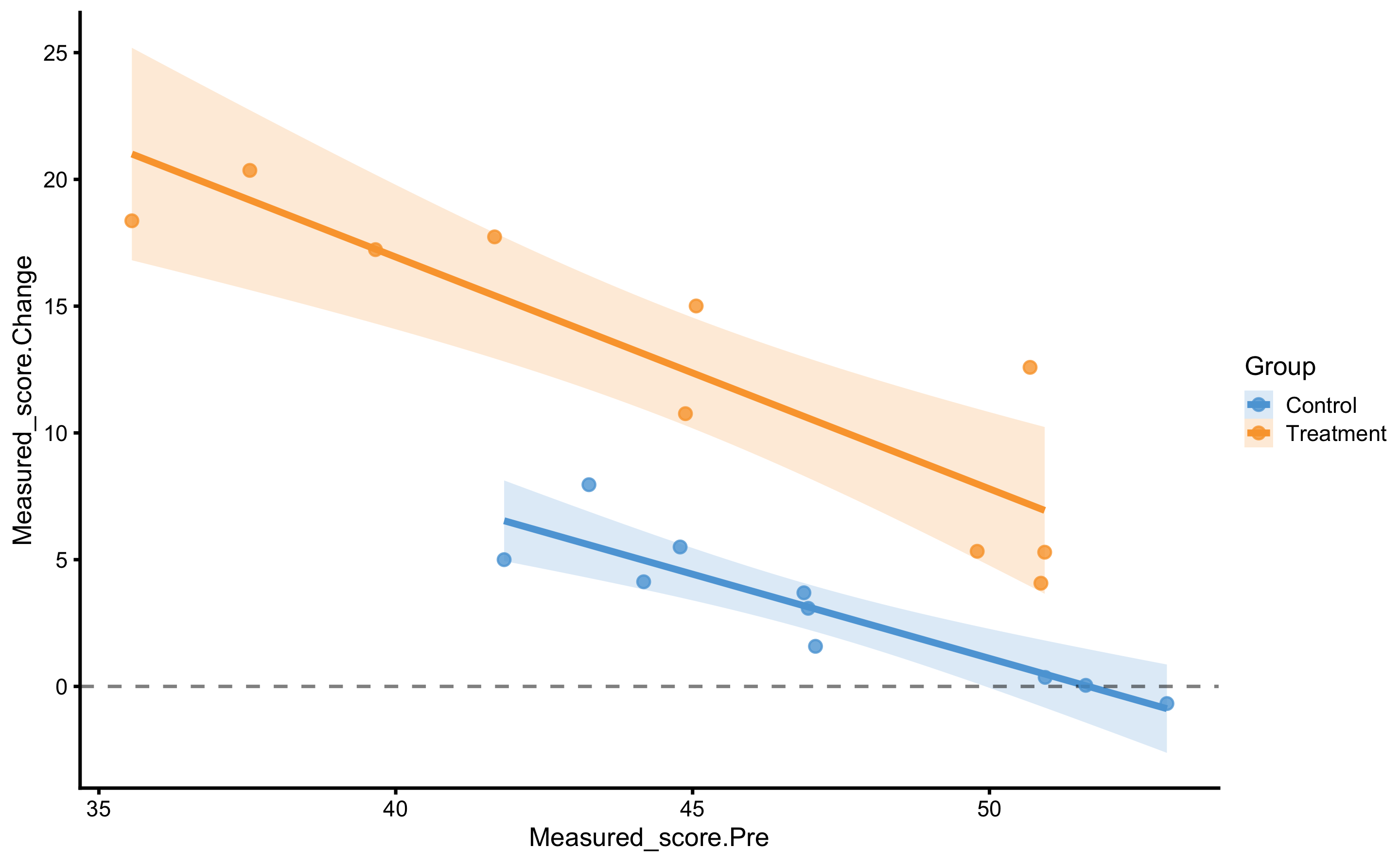
From these two graph we can see that as one has higher Pre-test, change scores gets smaller (i.e. effect decreases).
Let’s plot the 1RM strength relationship to Post-test:
ggplot(
  RCT_data,
  aes(x = Squat_1RM_relative, y = Measured_score.Post, color = Group, fill = Group)
) +
  theme_cowplot(8) +
  geom_smooth(method = "lm", se = TRUE, alpha = 0.2) +
  geom_point(alpha = 0.8) +
  scale_color_manual(values = c(Treatment = "#FAA43A", Control = "#5DA5DA")) +
  scale_fill_manual(values = c(Treatment = "#FAA43A", Control = "#5DA5DA"))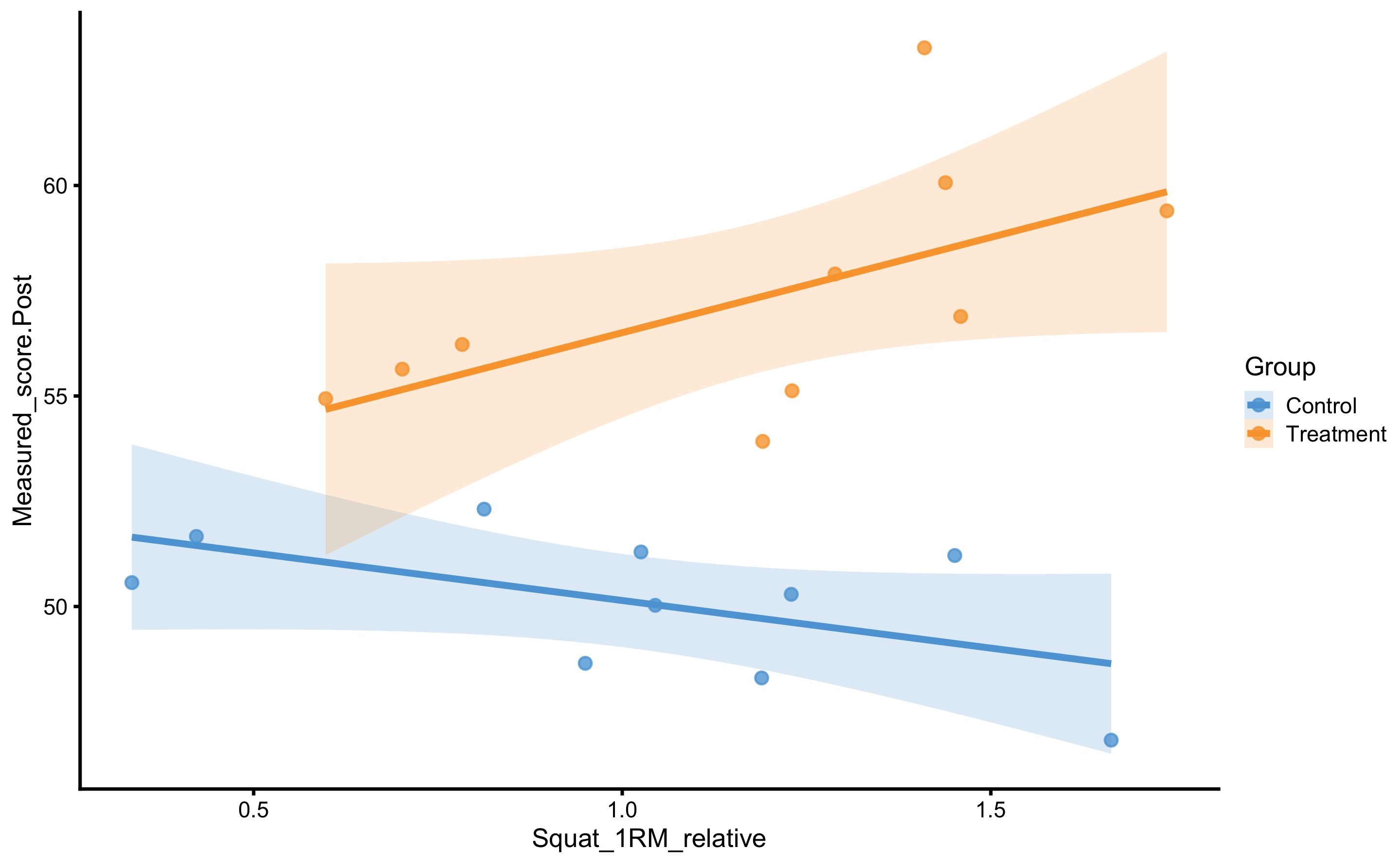
As can be seen from the figure, there is interaction between 1RM and group (the lines are not parallel). Let’s check with the change score:
ggplot(
  RCT_data,
  aes(x = Squat_1RM_relative, y = Measured_score.Change, color = Group, fill = Group)
) +
  theme_cowplot(8) +
  geom_smooth(method = "lm", se = TRUE, alpha = 0.2) +
  geom_hline(yintercept = 0, linetype = "dashed", alpha = 0.5) +
  geom_point(alpha = 0.8) +
  scale_color_manual(values = c(Treatment = "#FAA43A", Control = "#5DA5DA")) +
  scale_fill_manual(values = c(Treatment = "#FAA43A", Control = "#5DA5DA"))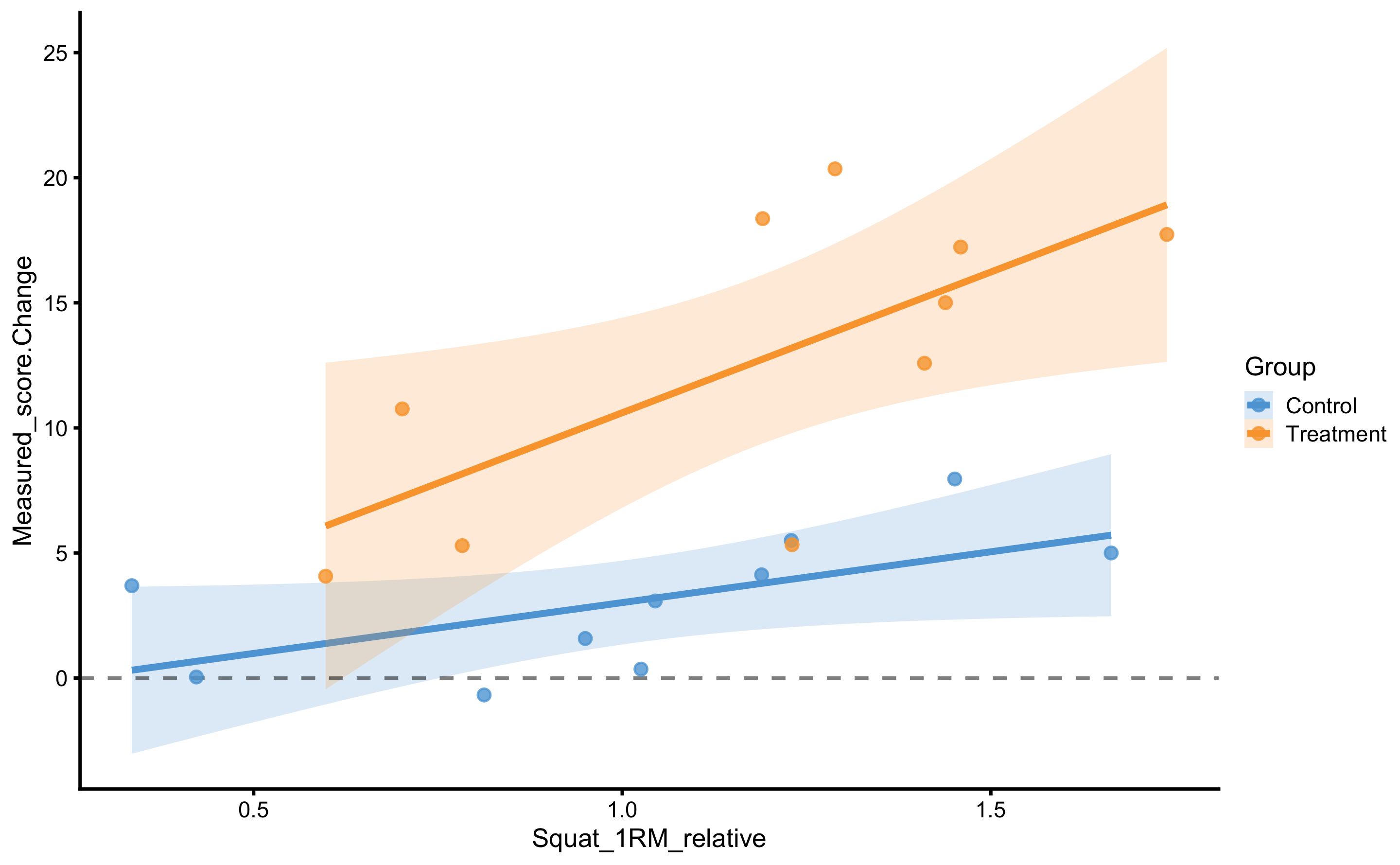
With change score we have controlled for Pre-test, which gives us information that the stronger someone is, the higher the improvement. This is even more evident for the Treatment group.
Let’s do the usual analysis and check the effects. Let’s first perform the method of the differences (which uses change score mean and SD):
simple_RCT <- bmbstats::RCT_analysis(
  data = RCT_data,
  group = "Group",
  treatment_label = "Treatment",
  control_label = "Control",
  pre_test = "Measured_score.Pre",
  post_test = "Measured_score.Post",
  SESOI_lower = -5,
  SESOI_upper = 5,
  estimator_function = bmbstats::RCT_estimators_simple,
  control = model_control(seed = 1667)
)
#> [1] "All values of t are equal to  5 \n Cannot calculate confidence intervals"
#> [1] "All values of t are equal to  10 \n Cannot calculate confidence intervals"


simple_RCT
#> Bootstrap with 2000 resamples and 95% bca confidence intervals.
#>
#>                   estimator       value      lower       upper
#>                 SESOI lower -5.00000000         NA          NA
#>                 SESOI upper  5.00000000         NA          NA
#>                 SESOI range 10.00000000         NA          NA
#>           Systematic effect  9.60660366 5.36900820 13.44947544
#>               Random effect  5.39012073 3.51072089  6.92558325
#>  Systematic effect to SESOI  0.96066037 0.53690082  1.34494754
#>      SESOI to Random effect  1.85524601 1.43972066  3.06650272
#>                      pLower  0.01200102 0.00037884  0.05838599
#>                 pEquivalent  0.19545959 0.02005083  0.46036640
#>                     pHigher  0.79253939 0.46809992  0.97792031
From our DGP we know that there is no random treatment effect, but only systematic treatment effect depending on the Pre-test and relative strength levels. But with this analysis we do not know that and we use only mean change to estimate treatment effects, and all the residuals around the mean (i.e. total variance) are assumed to be random error. This is unexplained variance (by this model). But we do know we can explain this variance with better model specification.
If we use linear regression model (using bmbstats::RCT_estimators_lm), we will address the effect of the Pre-test on the Post-test. But before, let’s just show model coefficients:
model6 <- lm(
  Measured_score.Post ~ Measured_score.Pre + Group,
  RCT_data
)

summary(model6)
#>
#> Call:
#> lm(formula = Measured_score.Post ~ Measured_score.Pre + Group,
#>     data = RCT_data)
#>
#> Residuals:
#>     Min      1Q  Median      3Q     Max
#> -3.3819 -1.7924  0.4125  1.3648  4.9797
#>
#> Coefficients:
#>                    Estimate Std. Error t value Pr(>|t|)
#> (Intercept)         42.6606     5.2220   8.169 2.74e-07 ***
#> Measured_score.Pre   0.1584     0.1099   1.441    0.168
#> GroupTreatment       7.5994     1.0578   7.184 1.53e-06 ***
#> ---
#> Signif. codes:  0 '***' 0.001 '**' 0.01 '*' 0.05 '.' 0.1 ' ' 1
#>
#> Residual standard error: 2.291 on 17 degrees of freedom
#> Multiple R-squared:  0.7527, Adjusted R-squared:  0.7236
#> F-statistic: 25.87 on 2 and 17 DF,  p-value: 6.963e-06
Visually, this model looks like this:
RCT_data$.pred <- predict(
  model6,
  newdata = RCT_data
)

ggplot(
  RCT_data,
  aes(x = Measured_score.Pre, y = Measured_score.Post, color = Group, fill = Group)
) +
  theme_cowplot(8) +
  geom_abline(slope = 1, linetype = "dashed") +
  geom_point(alpha = 0.8) +
  geom_line(aes(y = .pred)) +
  scale_color_manual(values = c(Treatment = "#FAA43A", Control = "#5DA5DA")) +
  scale_fill_manual(values = c(Treatment = "#FAA43A", Control = "#5DA5DA"))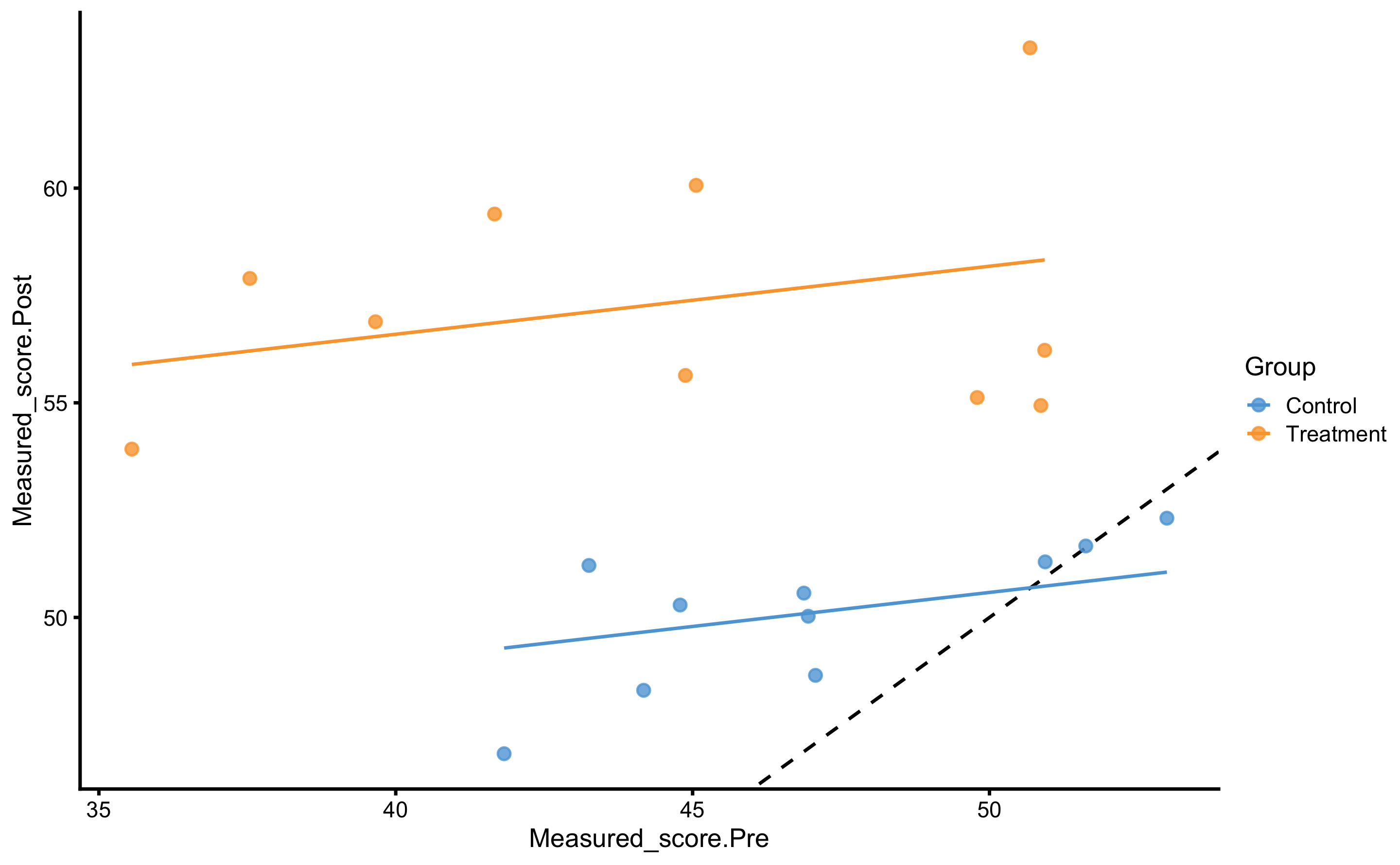
Estimated random treatment effect is equal to:
SD_summary <- RCT_data %>%
  mutate(.resid = residuals(model6)) %>%
  group_by(Group) %>%
  summarise(`Residual SD` = sd(.resid))


sqrt(SD_summary$`Residual SD`[2]^2 - SD_summary$`Residual SD`[1]^2)
#> [1] 2.521028
Now, let’s run this model using the bmbstats::RCT_estimators_lm and bmbstats::RCT_analysis:
regression_RCT <- bmbstats::RCT_analysis(
  data = RCT_data,
  group = "Group",
  treatment_label = "Treatment",
  control_label = "Control",
  pre_test = "Measured_score.Pre",
  post_test = "Measured_score.Post",
  SESOI_lower = -5,
  SESOI_upper = 5,
  estimator_function = bmbstats::RCT_estimators_lm,
  control = model_control(seed = 1667)
)
#> [1] "All values of t are equal to  5 \n Cannot calculate confidence intervals"
#> [1] "All values of t are equal to  10 \n Cannot calculate confidence intervals"


regression_RCT
#> Bootstrap with 2000 resamples and 95% bca confidence intervals.
#>
#>                   estimator         value         lower      upper
#>                 SESOI lower -5.000000e+00            NA         NA
#>                 SESOI upper  5.000000e+00            NA         NA
#>                 SESOI range  1.000000e+01            NA         NA
#>           Systematic effect  7.599370e+00  5.559460e+00 10.4054050
#>               Random effect  2.521028e+00  1.281688e+00  3.7842396
#>  Systematic effect to SESOI  7.599370e-01  5.559460e-01  1.0405405
#>      SESOI to Random effect  3.966636e+00 -2.288091e+01  9.9649843
#>                      pLower  3.995354e-05  7.377399e-10  1.0000000
#>                 pEquivalent  1.576864e-01  2.068126e-03  0.4686692
#>                     pHigher  8.422736e-01  3.994218e-05  0.9902346
Let’s plot the estimated from the method of differences and linear regression model for easier comparison:
compare_methods <- rbind(
  data.frame(method = "differences", simple_RCT$estimators),
  data.frame(method = "linear regression", regression_RCT$estimators)
)


ggplot(
  compare_methods,
  aes(y = method, x = value)
) +
  theme_bw(8) +
  geom_errorbarh(aes(xmax = upper, xmin = lower),
    color = "black",
    height = 0
  ) +
  geom_point() +
  xlab("") +
  ylab("") +
  facet_wrap(~estimator, scales = "free_x")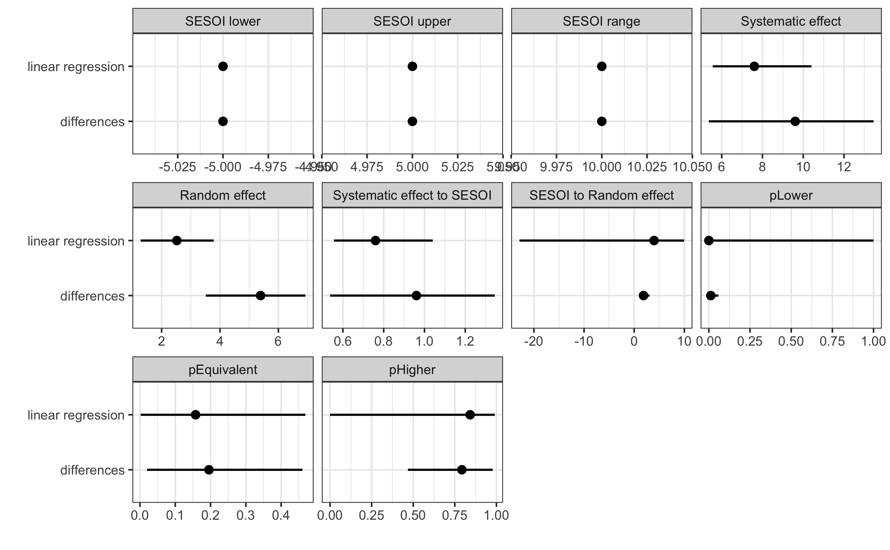
Please note that the estimated systematic treatment effect is smaller for the linear regression method compared to method of differences. It is the opposite for the random treatment effect estimate. This is because linear regression method estimates the effect of the group while controlling for the Pre-test.
Let’s now add relative 1RM strength to the mix:
model7 <- lm(
  Measured_score.Post ~ Measured_score.Pre + Squat_1RM_relative + Group,
  RCT_data
)

summary(model7)
#>
#> Call:
#> lm(formula = Measured_score.Post ~ Measured_score.Pre + Squat_1RM_relative +
#>     Group, data = RCT_data)
#>
#> Residuals:
#>     Min      1Q  Median      3Q     Max
#> -3.6732 -1.3602  0.1547  1.5569  3.7951
#>
#> Coefficients:
#>                    Estimate Std. Error t value Pr(>|t|)
#> (Intercept)         35.2743     6.7717   5.209 8.61e-05 ***
#> Measured_score.Pre   0.2621     0.1231   2.128   0.0492 *
#> Squat_1RM_relative   2.4779     1.5351   1.614   0.1260
#> GroupTreatment       7.4215     1.0171   7.297 1.79e-06 ***
#> ---
#> Signif. codes:  0 '***' 0.001 '**' 0.01 '*' 0.05 '.' 0.1 ' ' 1
#>
#> Residual standard error: 2.19 on 16 degrees of freedom
#> Multiple R-squared:  0.7873, Adjusted R-squared:  0.7474
#> F-statistic: 19.74 on 3 and 16 DF,  p-value: 1.259e-05
Please notice the slightly improved RSE of this model (indicating better model fit). Let’s check the estimate random treatment effect:
SD_summary <- RCT_data %>%
  mutate(.resid = residuals(model7)) %>%
  group_by(Group) %>%
  summarise(`Residual SD` = sd(.resid))


sqrt(SD_summary$`Residual SD`[2]^2 - SD_summary$`Residual SD`[1]^2)
#> [1] 1.59975
This implies that with this model we were able to explain more of the treatment effect. But we do know there is interaction between Group and relative 1RM. We can model that:
model8 <- lm(
  Measured_score.Post ~
    Measured_score.Pre + Squat_1RM_relative + Squat_1RM_relative:Group + Group,
  # OR we can specify the model with this
  # Measured_score.Post ~ Measured_score.Pre + Squat_1RM_relative * Group
  RCT_data
)

summary(model8)
#>
#> Call:
#> lm(formula = Measured_score.Post ~ Measured_score.Pre + Squat_1RM_relative +
#>     Squat_1RM_relative:Group + Group, data = RCT_data)
#>
#> Residuals:
#>     Min      1Q  Median      3Q     Max
#> -3.8832 -0.8725 -0.0257  0.9302  2.8875
#>
#> Coefficients:
#>                                   Estimate Std. Error t value Pr(>|t|)
#> (Intercept)                       38.07464    5.35343   7.112 3.55e-06 ***
#> Measured_score.Pre                 0.26809    0.09618   2.787  0.01381 *
#> Squat_1RM_relative                -0.56615    1.50382  -0.376  0.71183
#> GroupTreatment                    -0.20765    2.41029  -0.086  0.93248
#> Squat_1RM_relative:GroupTreatment  6.89774    2.05750   3.352  0.00436 **
#> ---
#> Signif. codes:  0 '***' 0.001 '**' 0.01 '*' 0.05 '.' 0.1 ' ' 1
#>
#> Residual standard error: 1.71 on 15 degrees of freedom
#> Multiple R-squared:  0.8784, Adjusted R-squared:  0.846
#> F-statistic: 27.09 on 4 and 15 DF,  p-value: 1.039e-06
RSE of this model improved even further. Let’s calculate the random treatment effect:
SD_summary <- RCT_data %>%
  mutate(.resid = residuals(model8)) %>%
  group_by(Group) %>%
  summarise(`Residual SD` = sd(.resid))


sqrt(SD_summary$`Residual SD`[2]^2 - SD_summary$`Residual SD`[1]^2)
#> [1] 1.476142
We managed to explain mode of the treatment effect (i.e. reduce the random component), but how do we not estimate the systematic effect? Now we have interaction term, and we introduced indirect effect of the Group:1RM, so we cannot simply quantify it with a single number.
But maybe the predictive perspective can help?
16.9 Prediction perspective 3
Before analyzing the most complex model specification, let’s build from the ground-up again using baseline model first. This model predicts Post-test to be the same for everyone using Group as predictor. This model is useful since it gives us the worst prediction we can use to judge the other models.
Since we are going to perform same modeling using different specification, to avoid repeating the code (which I have done on purpose thorough this book, but will avoid doing here), I will write down the function:
model_RCT <- function(formula) {
  model <- cv_model(
    formula,
    RCT_data,
    SESOI_lower = -5,
    SESOI_upper = 5,
    control = model_control(
      seed = 1667,
      cv_folds = 5,
      cv_repeats = 10,
      cv_strata = factor(RCT_data$Group)
    )
  )

  RCT <- RCT_predict(
    model,
    new_data = RCT_data,
    outcome = "Measured_score.Post",
    group = "Group",
    treatment_label = "Treatment",
    control_label = "Control",
    subject_label = RCT_data$Athlete
  )

  return(RCT)
}
Here is our baseline model:
base_model <- model_RCT(Measured_score.Post ~ Group)

base_model
#> Training data consists of 2 predictors and 20 observations.
#> Cross-Validation of the model was performed using 10 repeats of 5 folds.
#>
#> Model performance:
#>
#>         metric      training training.pooled testing.pooled          mean         SD
#>            MBE -4.618506e-15    1.634262e-15   1.634259e-15  1.634238e-15 1.33279182
#>            MAE  1.793742e+00    1.768937e+00   1.997720e+00  1.997720e+00 0.55544631
#>           RMSE  2.238021e+00    2.206270e+00   2.505740e+00  2.393620e+00 0.74868547
#>           PPER  9.577526e-01    9.762111e-01   9.520871e-01  8.549957e-01 0.08929827
#>  SESOI to RMSE  4.468233e+00    4.532536e+00   3.990837e+00  4.591613e+00 1.42736849
#>      R-squared  7.224490e-01    7.302684e-01   6.520744e-01  6.595240e-01 0.32999136
#>         MinErr -5.933469e+00   -6.532374e+00  -7.016430e+00 -2.794574e+00 2.16480138
#>         MaxErr  3.414524e+00    3.926733e+00   4.141234e+00  2.385040e+00 1.21855651
#>      MaxAbsErr  5.933469e+00    6.532374e+00   7.016430e+00  3.768324e+00 1.58419875
#>         min       max
#>  -2.5926409 2.7658984
#>   1.0781811 3.3474423
#>   1.1928031 4.0973536
#>   0.6560171 0.9718218
#>   2.4405997 8.3836132
#>  -0.5542973 0.9646862
#>  -7.0164300 2.0578483
#>  -0.2376657 4.1412343
#>   1.4647768 7.0164300
#>
#> Individual model results:
#>
#>     subject     group observed predicted    residual  magnitude counterfactual      pITE
#>  Athlete 01 Treatment 53.92165  57.33617  3.41452429 Equivalent       50.11469 -7.221484
#>  Athlete 02   Control 48.65099  50.11469  1.46369772 Equivalent       57.33617  7.221484
#>  Athlete 03 Treatment 60.06640  57.33617 -2.73022311 Equivalent       50.11469 -7.221484
#>  Athlete 04   Control 51.66451  50.11469 -1.54981912 Equivalent       57.33617  7.221484
#>  Athlete 05 Treatment 56.88816  57.33617  0.44801588 Equivalent       50.11469 -7.221484
#>  Athlete 06   Control 52.31237  50.11469 -2.19768413 Equivalent       57.33617  7.221484
#>  Athlete 07 Treatment 54.93702  57.33617  2.39915590 Equivalent       50.11469 -7.221484
#>  Athlete 08   Control 51.29489  50.11469 -1.18019529 Equivalent       57.33617  7.221484
#>  Athlete 09 Treatment 63.26964  57.33617 -5.93346853      Lower       50.11469 -7.221484
#>  Athlete 10   Control 50.28937  50.11469 -0.17467663 Equivalent       57.33617  7.221484
#>  Athlete 11 Treatment 59.39720  57.33617 -2.06102088 Equivalent       50.11469 -7.221484
#>  Athlete 12   Control 50.02810  50.11469  0.08658834 Equivalent       57.33617  7.221484
#>  Athlete 13 Treatment 55.63766  57.33617  1.69851405 Equivalent       50.11469 -7.221484
#>  Athlete 14   Control 46.82518  50.11469  3.28950733 Equivalent       57.33617  7.221484
#>  Athlete 15 Treatment 57.89749  57.33617 -0.56131425 Equivalent       50.11469 -7.221484
#>  Athlete 16   Control 50.56725  50.11469 -0.45256087 Equivalent       57.33617  7.221484
#>  Athlete 17 Treatment 55.12290  57.33617  2.21327604 Equivalent       50.11469 -7.221484
#>  Athlete 18   Control 48.30309  50.11469  1.81159973 Equivalent       57.33617  7.221484
#>  Athlete 19 Treatment 56.22363  57.33617  1.11254061 Equivalent       50.11469 -7.221484
#>  Athlete 20   Control 51.21115  50.11469 -1.09645708 Equivalent       57.33617  7.221484
#>  pITE_magnitude
#>           Lower
#>          Higher
#>           Lower
#>          Higher
#>           Lower
#>          Higher
#>           Lower
#>          Higher
#>           Lower
#>          Higher
#>           Lower
#>          Higher
#>           Lower
#>          Higher
#>           Lower
#>          Higher
#>           Lower
#>          Higher
#>           Lower
#>          Higher
#>
#> Summary of residuals per RCT group:
#>
#>      group          mean       SD
#>    Control -2.842214e-15 1.709932
#>  Treatment -6.394885e-15 2.864728
#>
#> Summary of counterfactual effects of RCT group:
#>
#>      group      pATE pVTE
#>  Treatment -7.221484    0
#>    Control  7.221484    0
#>     pooled  7.221484    0
#>
#> Treatment effect summary
#>
#> Average Treatment effect:  7.221484
#> Variable Treatment effect:  0
#> Random Treatment effect:  2.298433
Let’s plot key model predictions (individual and counterfactual).
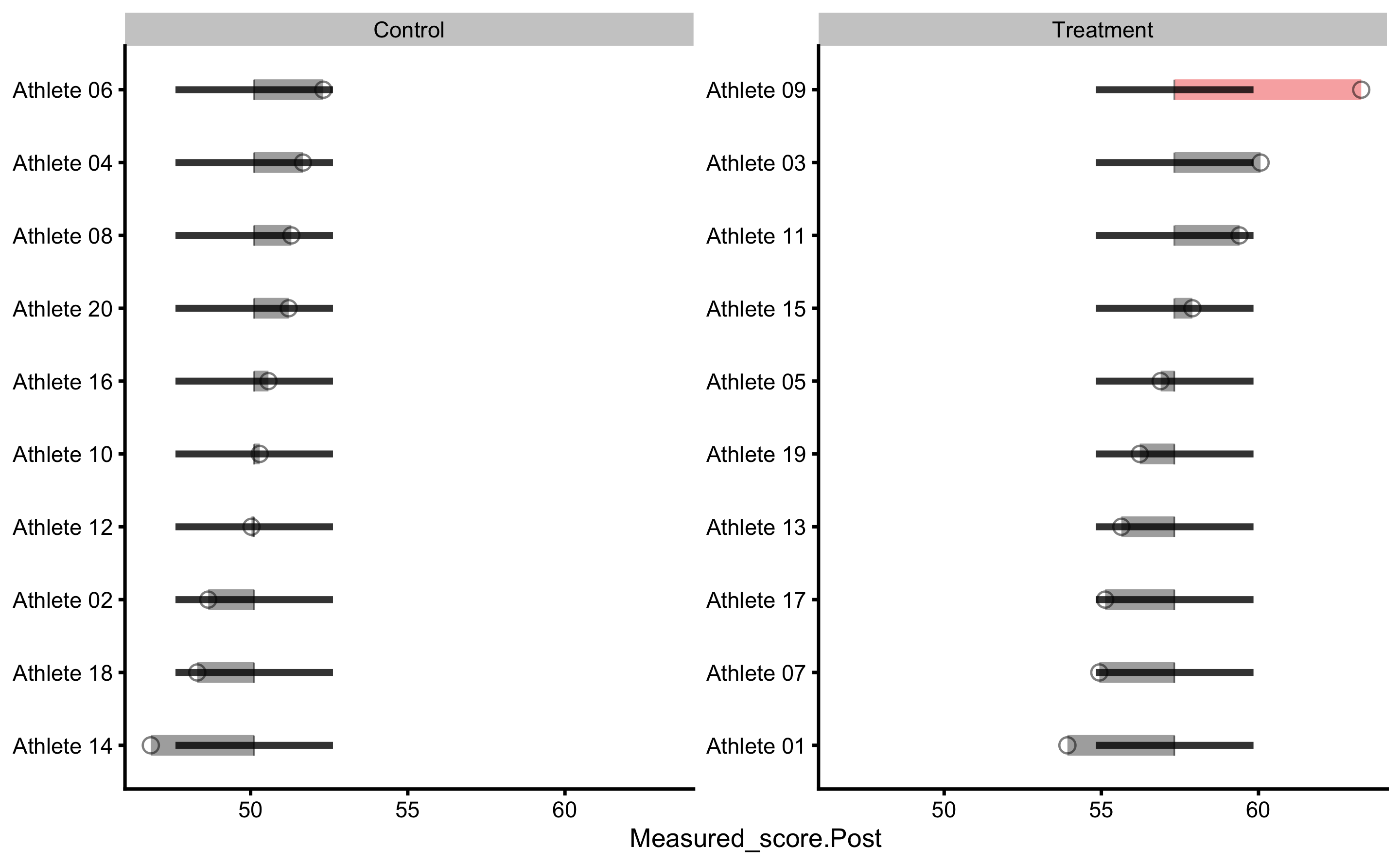
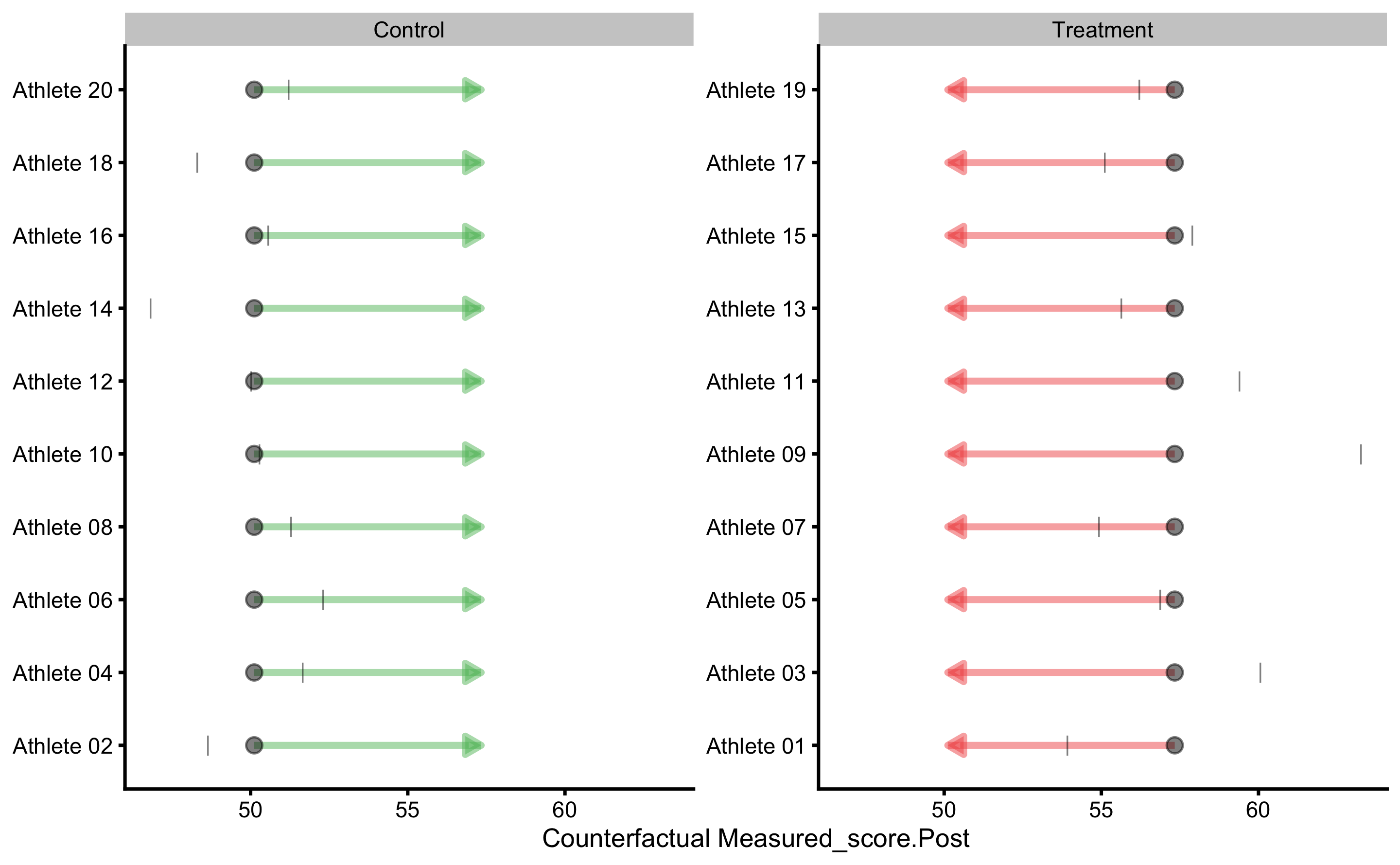
As can be seen, base model predict the same Post-test scores for each athlete (depending on the group).
Our next model is the one that uses Pre-test and Group. Let’s call it pre_test_model (please note that this is the model used in bmbstats::RCT_estimators_lm function):
pre_test_model <- model_RCT(Measured_score.Post ~ Group + Measured_score.Pre)

pre_test_model
#> Training data consists of 3 predictors and 20 observations.
#> Cross-Validation of the model was performed using 10 repeats of 5 folds.
#>
#> Model performance:
#>
#>         metric      training training.pooled testing.pooled        mean         SD
#>            MBE -1.385555e-14    3.774758e-15     0.03197143  0.03197143 1.25159476
#>            MAE  1.757354e+00    1.700865e+00     2.04500207  2.04500207 0.53059190
#>           RMSE  2.112647e+00    2.066468e+00     2.51137986  2.43165066 0.63415044
#>           PPER  9.675019e-01    9.841744e-01     0.95158915  0.84684948 0.07383527
#>  SESOI to RMSE  4.733399e+00    4.839174e+00     3.98187473  4.44664689 1.40990552
#>      R-squared  7.526750e-01    7.633690e-01     0.65056316  0.63480891 0.32450934
#>         MinErr -4.979659e+00   -5.620519e+00    -6.48925129 -2.73668942 1.95426062
#>         MaxErr  3.381897e+00    4.723784e+00     4.36811806  2.71096150 1.23032364
#>      MaxAbsErr  4.979659e+00    5.620519e+00     6.48925129  3.85285271 1.30595427
#>         min       max
#>  -2.5288076 2.8367663
#>   0.8621495 3.2662051
#>   1.0726499 3.8740486
#>   0.6842390 0.9746472
#>   2.5812789 9.3227066
#>  -0.7834415 0.9507508
#>  -6.4892513 1.9406012
#>  -0.6916705 4.3681181
#>   1.9061280 6.4892513
#>
#> Individual model results:
#>
#>     subject     group observed predicted    residual  magnitude counterfactual     pITE
#>  Athlete 01 Treatment 53.92165  55.89316  1.97150648 Equivalent       48.29379 -7.59937
#>  Athlete 02   Control 48.65099  50.11805  1.46705656 Equivalent       57.71742  7.59937
#>  Athlete 03 Treatment 60.06640  57.39899 -2.66741213 Equivalent       49.79962 -7.59937
#>  Athlete 04   Control 51.66451  50.83931 -0.82520345 Equivalent       58.43868  7.59937
#>  Athlete 05 Treatment 56.88816  56.54332 -0.34484151 Equivalent       48.94395 -7.59937
#>  Athlete 06   Control 52.31237  51.05577 -1.25660375 Equivalent       58.65514  7.59937
#>  Athlete 07 Treatment 54.93702  58.31892  3.38189720 Equivalent       50.71955 -7.59937
#>  Athlete 08   Control 51.29489  50.73095 -0.56393813 Equivalent       58.33032  7.59937
#>  Athlete 09 Treatment 63.26964  58.28998 -4.97965920 Equivalent       50.69061 -7.59937
#>  Athlete 10   Control 50.28937  49.75682 -0.53254676 Equivalent       57.35619  7.59937
#>  Athlete 11 Treatment 59.39720  56.86111 -2.53609024 Equivalent       49.26174 -7.59937
#>  Athlete 12   Control 50.02810  50.09865  0.07054839 Equivalent       57.69802  7.59937
#>  Athlete 13 Treatment 55.63766  57.37036  1.73269990 Equivalent       49.77099 -7.59937
#>  Athlete 14   Control 46.82518  49.28717  2.46198498 Equivalent       56.88654  7.59937
#>  Athlete 15 Treatment 57.89749  56.20799 -1.68949873 Equivalent       48.60862 -7.59937
#>  Athlete 16   Control 50.56725  50.08713 -0.48012312 Equivalent       57.68650  7.59937
#>  Athlete 17 Treatment 55.12290  58.14891  3.02601000 Equivalent       50.54954 -7.59937
#>  Athlete 18   Control 48.30309  49.65954  1.35644850 Equivalent       57.25891  7.59937
#>  Athlete 19 Treatment 56.22363  58.32902  2.10538825 Equivalent       50.72965 -7.59937
#>  Athlete 20   Control 51.21115  49.51352 -1.69762322 Equivalent       57.11289  7.59937
#>  pITE_magnitude
#>           Lower
#>          Higher
#>           Lower
#>          Higher
#>           Lower
#>          Higher
#>           Lower
#>          Higher
#>           Lower
#>          Higher
#>           Lower
#>          Higher
#>           Lower
#>          Higher
#>           Lower
#>          Higher
#>           Lower
#>          Higher
#>           Lower
#>          Higher
#>
#> Summary of residuals per RCT group:
#>
#>      group          mean       SD
#>    Control -1.136866e-14 1.334693
#>  Treatment -1.634257e-14 2.852540
#>
#> Summary of counterfactual effects of RCT group:
#>
#>      group     pATE         pVTE
#>  Treatment -7.59937 5.246187e-15
#>    Control  7.59937 2.254722e-15
#>     pooled  7.59937 3.992905e-15
#>
#> Treatment effect summary
#>
#> Average Treatment effect:  7.59937
#> Variable Treatment effect:  3.992905e-15
#> Random Treatment effect:  2.521028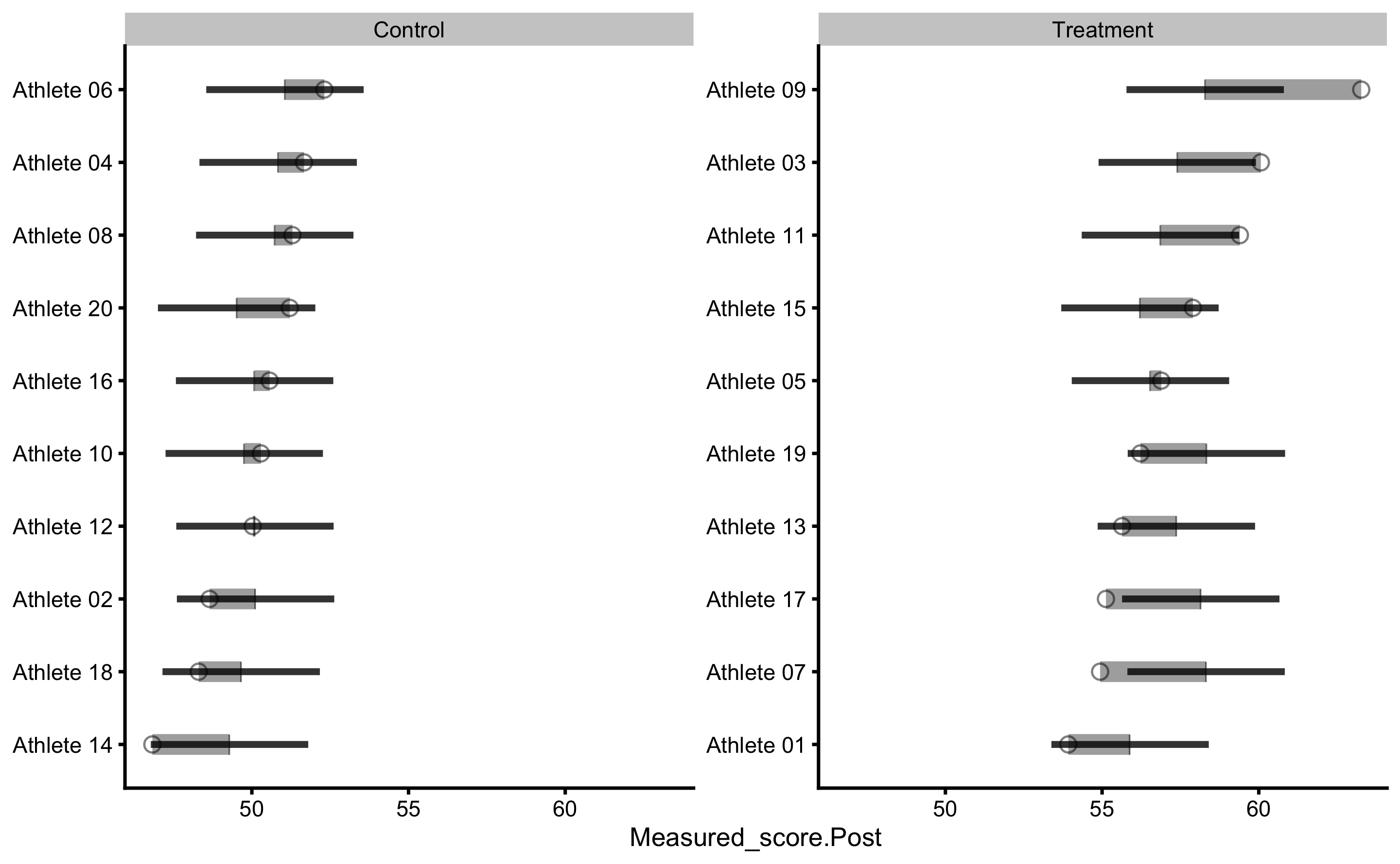
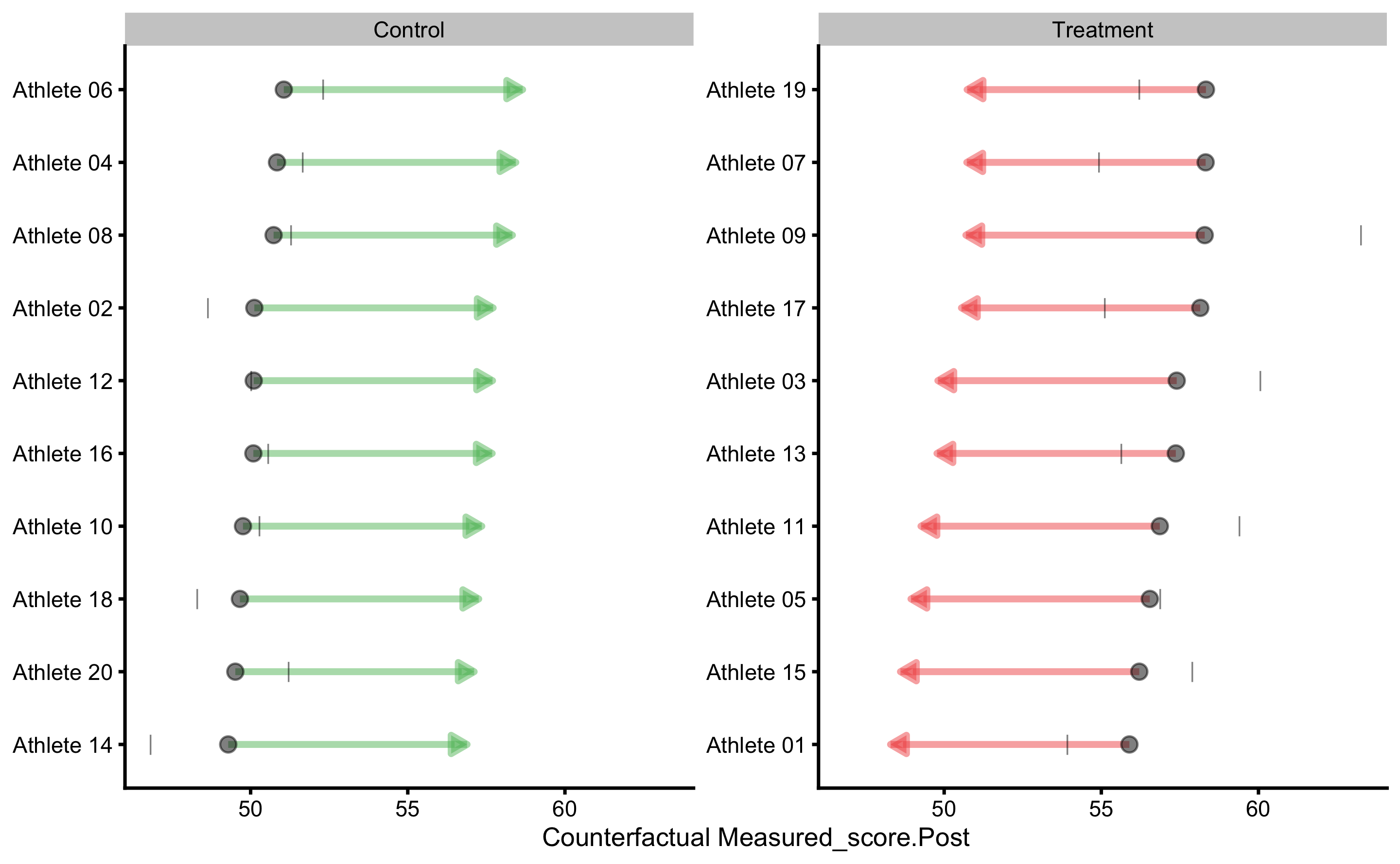
Additional plot we can do is the PDP+ICE for group predictor (i.e. treatment effect):
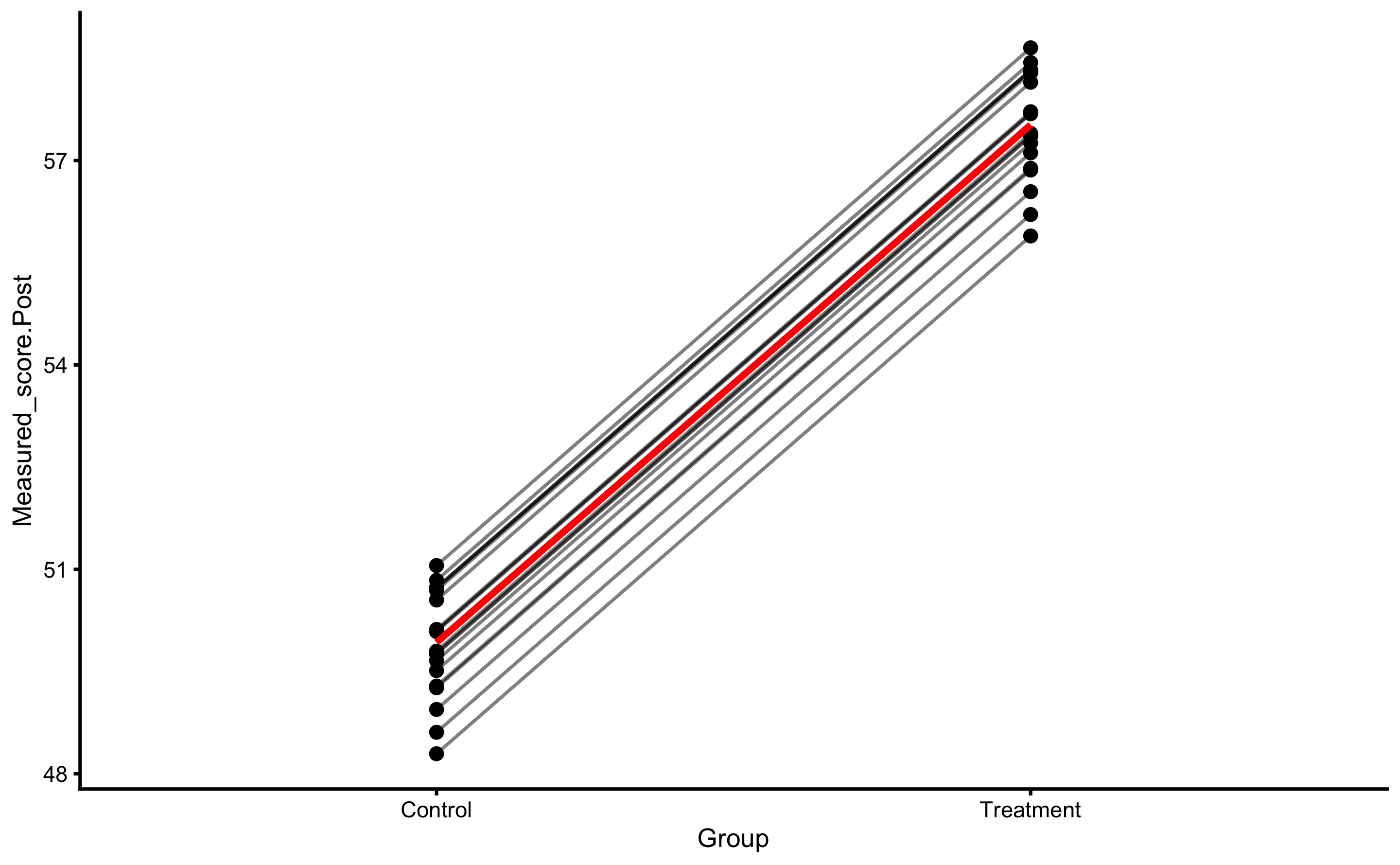
And also for the Pre-test predictor:
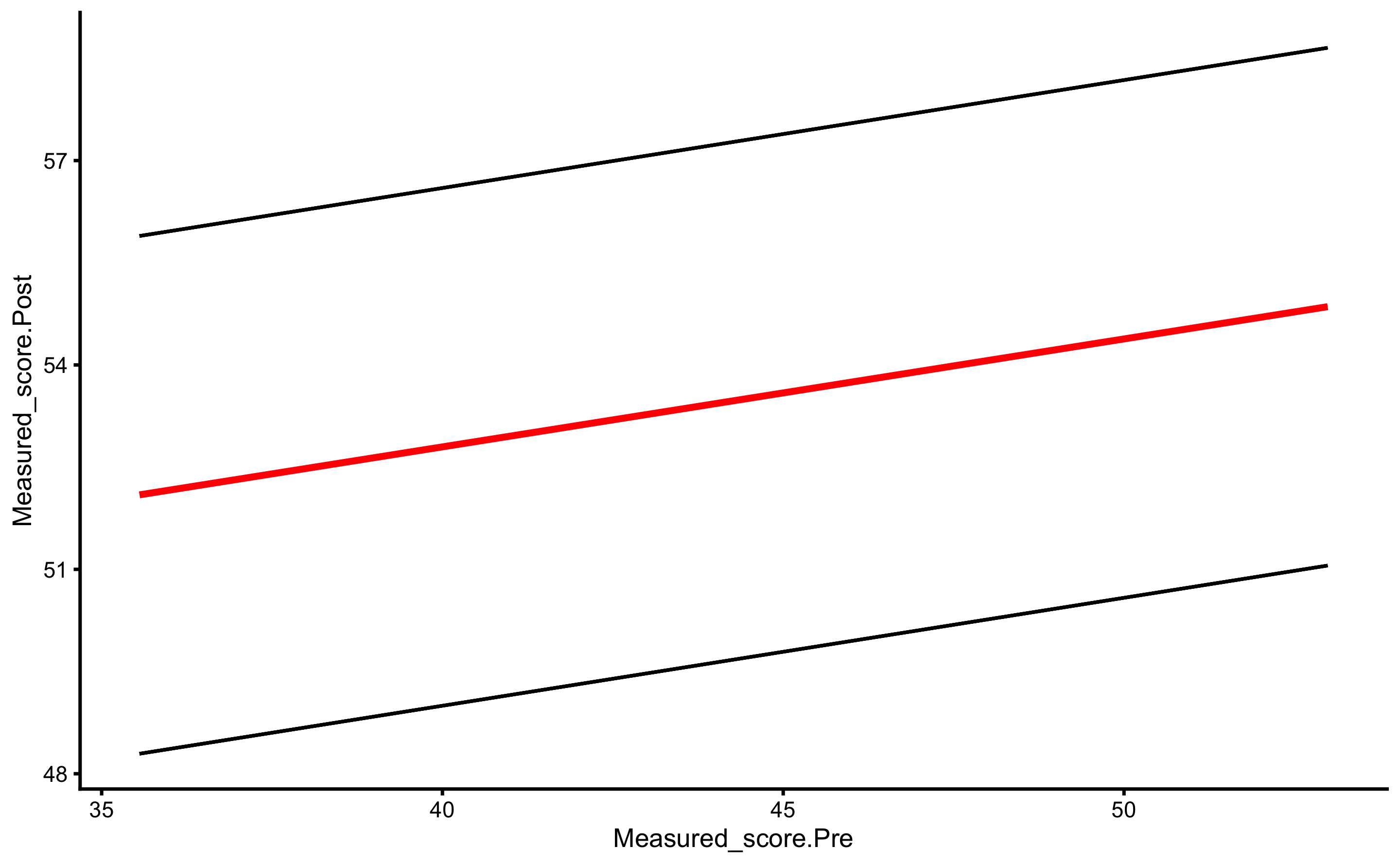
Next model adds additional predictor (covariate): relative squat 1RM:
covariate_model <- model_RCT(
  Measured_score.Post ~ Group + Measured_score.Pre + Squat_1RM_relative
  )

covariate_model
#> Training data consists of 4 predictors and 20 observations.
#> Cross-Validation of the model was performed using 10 repeats of 5 folds.
#>
#> Model performance:
#>
#>         metric      training training.pooled testing.pooled        mean         SD
#>            MBE -1.492140e-14    3.641497e-15    -0.04731864 -0.04731864 1.27184288
#>            MAE  1.609713e+00    1.560087e+00     1.99431750  1.99431750 0.67386685
#>           RMSE  1.959142e+00    1.895527e+00     2.51905179  2.40288524 0.76382791
#>           PPER  9.776803e-01    9.914518e-01     0.95090835  0.84667956 0.08174096
#>  SESOI to RMSE  5.104275e+00    5.275579e+00     3.96974768  5.02832487 3.49488784
#>      R-squared  7.873104e-01    8.008987e-01     0.64849202  0.58513228 0.56466111
#>         MinErr -3.795052e+00   -4.671246e+00    -6.30927941 -2.64672001 1.65641966
#>         MaxErr  3.673197e+00    4.356870e+00     5.13611940  2.81303001 1.68991662
#>      MaxAbsErr  3.795052e+00    4.671246e+00     6.30927941  3.84840058 1.32366331
#>         min        max
#>  -2.4388220  2.4598851
#>   0.3458090  3.4404583
#>   0.4106030  3.7642949
#>   0.6970788  0.9981811
#>   2.6565400 24.3544266
#>  -1.9362660  0.9784156
#>  -6.3092794  0.8127197
#>  -0.2922030  5.1361194
#>   0.7157490  6.3092794
#>
#> Individual model results:
#>
#>     subject     group observed predicted   residual  magnitude counterfactual      pITE
#>  Athlete 01 Treatment 53.92165  54.96555  1.0439001 Equivalent       47.54404 -7.421514
#>  Athlete 02   Control 48.65099  49.96562  1.3146319 Equivalent       57.38714  7.421514
#>  Athlete 03 Treatment 60.06640  58.07113 -1.9952645 Equivalent       50.64962 -7.421514
#>  Athlete 04   Control 51.66451  49.85167 -1.8128409 Equivalent       57.27318  7.421514
#>  Athlete 05 Treatment 56.88816  56.70667 -0.1814903 Equivalent       49.28515 -7.421514
#>  Athlete 06   Control 52.31237  51.17699 -1.1353824 Equivalent       58.59851  7.421514
#>  Athlete 07 Treatment 54.93702  57.50946  2.5724418 Equivalent       50.08795 -7.421514
#>  Athlete 08   Control 51.29489  51.16688 -0.1280040 Equivalent       58.58840  7.421514
#>  Athlete 09 Treatment 63.26964  59.47459 -3.7950523 Equivalent       52.05308 -7.421514
#>  Athlete 10   Control 50.28937  50.06036 -0.2290056 Equivalent       57.48188  7.421514
#>  Athlete 11 Treatment 59.39720  57.92560 -1.4715975 Equivalent       50.50408 -7.421514
#>  Athlete 12   Control 50.02810  50.16875  0.1406476 Equivalent       57.59026  7.421514
#>  Athlete 13 Treatment 55.63766  56.19778  0.5601237 Equivalent       48.77627 -7.421514
#>  Athlete 14   Control 46.82518  50.35886  3.5336766 Equivalent       57.78037  7.421514
#>  Athlete 15 Treatment 57.89749  55.72955 -2.1679347 Equivalent       48.30804 -7.421514
#>  Athlete 16   Control 50.56725  48.39034 -2.1769094 Equivalent       55.81186  7.421514
#>  Athlete 17 Treatment 55.12290  58.79610  3.6731974 Equivalent       51.37458 -7.421514
#>  Athlete 18   Control 48.30309  49.79992  1.4968326 Equivalent       57.22144  7.421514
#>  Athlete 19 Treatment 56.22363  57.98531  1.7616764 Equivalent       50.56380 -7.421514
#>  Athlete 20   Control 51.21115  50.20750 -1.0036463 Equivalent       57.62902  7.421514
#>  pITE_magnitude
#>           Lower
#>          Higher
#>           Lower
#>          Higher
#>           Lower
#>          Higher
#>           Lower
#>          Higher
#>           Lower
#>          Higher
#>           Lower
#>          Higher
#>           Lower
#>          Higher
#>           Lower
#>          Higher
#>           Lower
#>          Higher
#>           Lower
#>          Higher
#>
#> Summary of residuals per RCT group:
#>
#>      group          mean       SD
#>    Control -1.492135e-14 1.727747
#>  Treatment -1.492135e-14 2.354636
#>
#> Summary of counterfactual effects of RCT group:
#>
#>      group      pATE         pVTE
#>  Treatment -7.421514 5.617334e-15
#>    Control  7.421514 4.037713e-15
#>     pooled  7.421514 4.890290e-15
#>
#> Treatment effect summary
#>
#> Average Treatment effect:  7.421514
#> Variable Treatment effect:  4.89029e-15
#> Random Treatment effect:  1.59975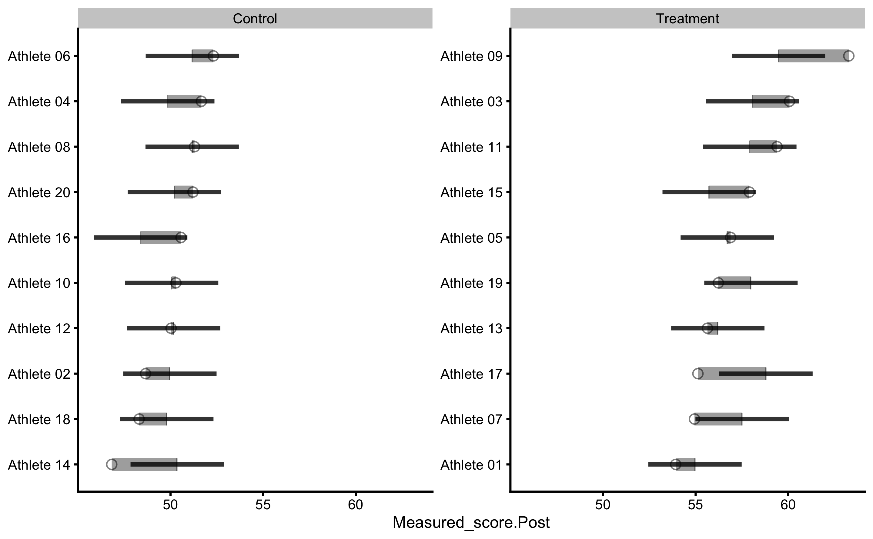
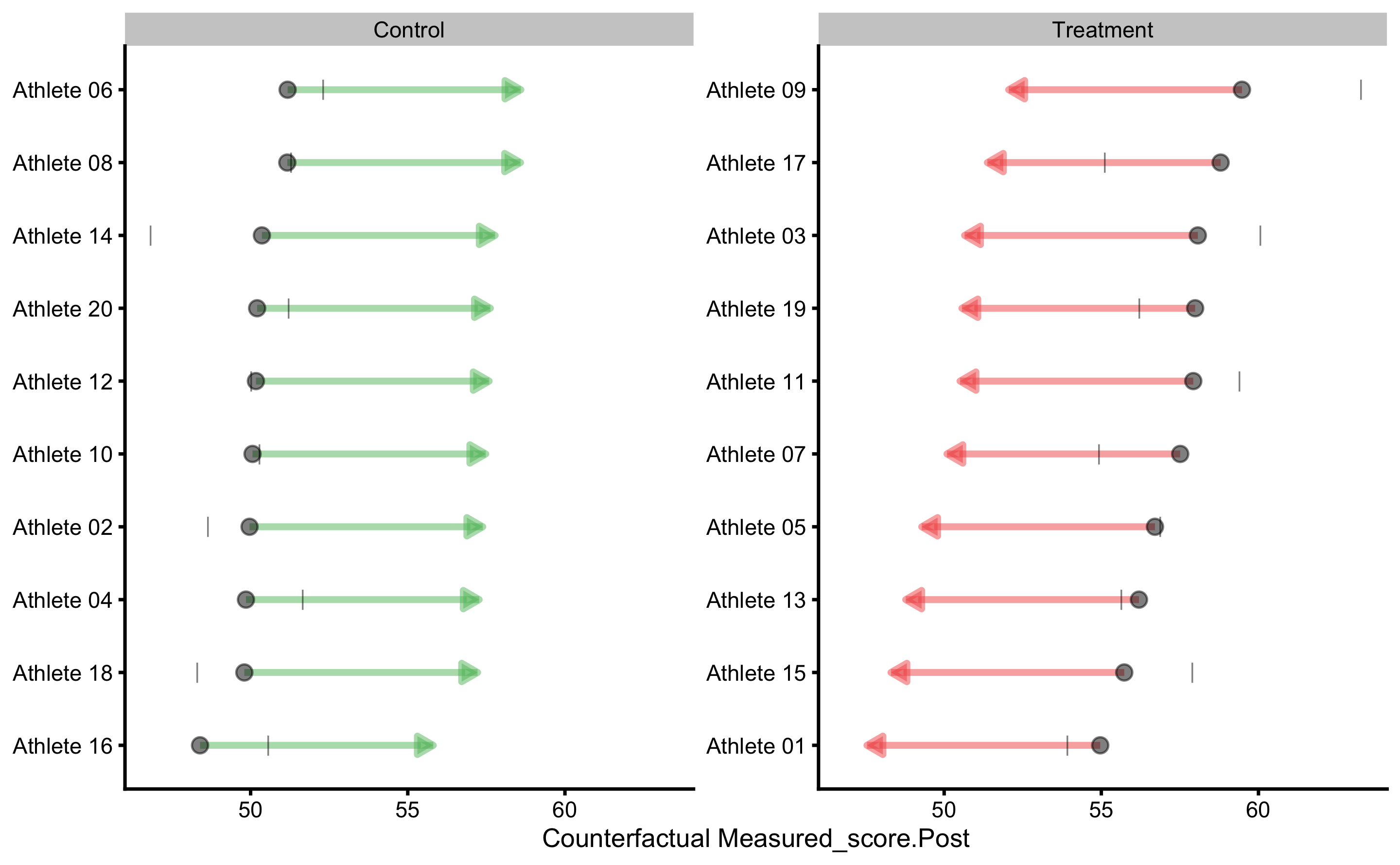
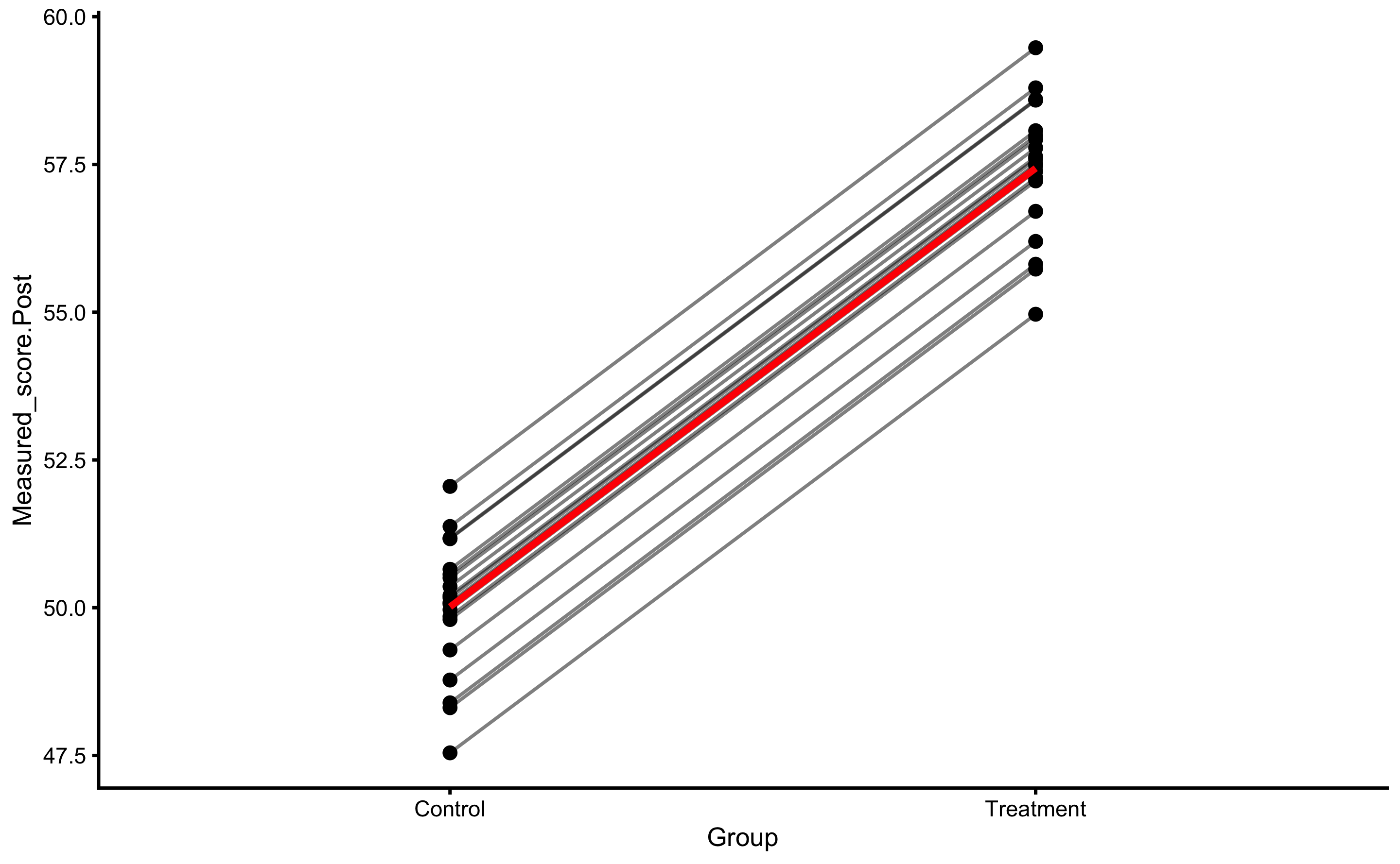
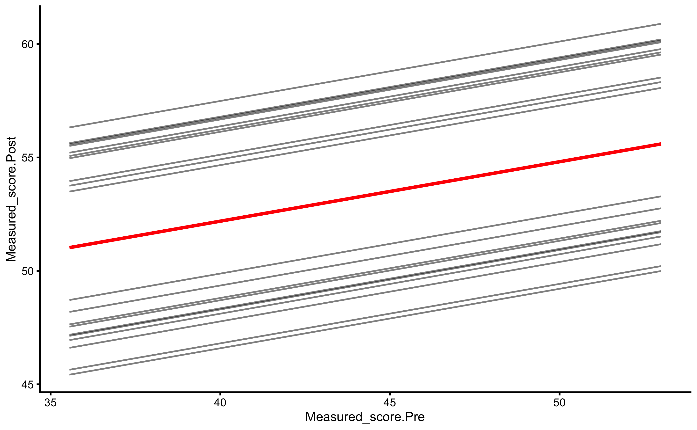
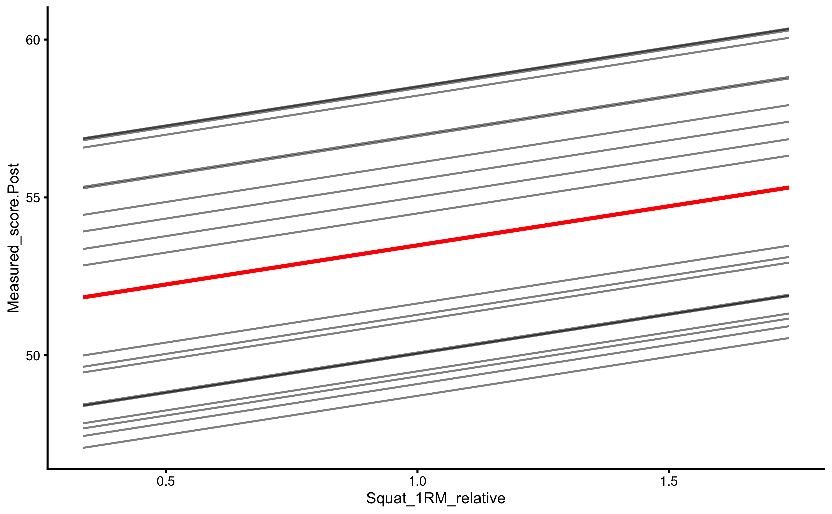
And the final model is the interaction model:
interaction_model <- model_RCT(
  Measured_score.Post ~ Group*Squat_1RM_relative + Measured_score.Pre
  )

interaction_model
#> Training data consists of 5 predictors and 20 observations.
#> Cross-Validation of the model was performed using 10 repeats of 5 folds.
#>
#> Model performance:
#>
#>         metric      training training.pooled testing.pooled        mean         SD
#>            MBE  2.486856e-15    5.107026e-15    -0.02897255 -0.02897255 0.96232473
#>            MAE  1.102035e+00    1.073541e+00     1.51448758  1.51448758 0.62541112
#>           RMSE  1.481278e+00    1.420252e+00     2.00731144  1.86964221 0.73799039
#>           PPER  9.961488e-01    9.995411e-01     0.98620762  0.90318747 0.07713261
#>  SESOI to RMSE  6.750926e+00    7.041003e+00     4.98178798  6.39845655 2.94071918
#>      R-squared  8.784129e-01    8.882249e-01     0.77676962  0.72661171 0.39233243
#>         MinErr -2.887520e+00   -3.387465e+00    -4.84781640 -2.22509568 1.45777723
#>         MaxErr  3.883197e+00    4.125618e+00     5.22505955  2.04804580 1.57273644
#>      MaxAbsErr  3.883197e+00    4.125618e+00     5.22505955  3.10011470 1.33675406
#>          min        max
#>  -2.10791777  2.0771169
#>   0.42250638  2.9228564
#>   0.62520553  3.2658803
#>   0.73706941  0.9955572
#>   3.06196160 15.9947402
#>  -1.30891277  0.9875223
#>  -4.84781640  1.2235186
#>   0.03320484  5.2250596
#>   1.05228122  5.2250596
#>
#> Individual model results:
#>
#>     subject     group observed predicted    residual  magnitude counterfactual       pITE
#>  Athlete 01 Treatment 53.92165  54.93714  1.01549088 Equivalent       46.93258  -8.004564
#>  Athlete 02   Control 48.65099  50.15570  1.50470919 Equivalent       56.49986   6.344157
#>  Athlete 03 Treatment 60.06640  59.05490 -1.01150268 Equivalent       49.34023  -9.714660
#>  Athlete 04   Control 51.66451  51.67481  0.01030262 Equivalent       54.38014   2.705324
#>  Athlete 05 Treatment 56.88816  57.73773  0.84957368 Equivalent       47.88067  -9.857066
#>  Athlete 06   Control 52.31237  51.82011 -0.49226674 Equivalent       57.21781   5.397698
#>  Athlete 07 Treatment 54.93702  55.28749  0.35047044 Equivalent       51.37291  -3.914577
#>  Athlete 08   Control 51.29489  51.15000 -0.14488443 Equivalent       58.01547   6.865468
#>  Athlete 09 Treatment 63.26964  60.38212 -2.88752039 Equivalent       50.86403  -9.518092
#>  Athlete 10   Control 50.28937  49.38628 -0.90309058 Equivalent       57.65772   8.271448
#>  Athlete 11 Treatment 59.39720  60.04667  0.64947349 Equivalent       48.26002 -11.786649
#>  Athlete 12   Control 50.02810  50.06914  0.04103265 Equivalent       57.06806   6.998928
#>  Athlete 13 Treatment 55.63766  54.34070 -1.29696009 Equivalent       49.70900  -4.631703
#>  Athlete 14   Control 46.82518  48.34585  1.52066587 Equivalent       59.61112  11.265266
#>  Athlete 15 Treatment 57.89749  56.09115 -1.80634311 Equivalent       47.40976  -8.681390
#>  Athlete 16   Control 50.56725  50.45161 -0.11564089 Equivalent       52.55310   2.101491
#>  Athlete 17 Treatment 55.12290  59.00610  3.88319663 Equivalent       50.72701  -8.279084
#>  Athlete 18   Control 48.30309  49.24440  0.94130869 Equivalent       57.23888   7.994484
#>  Athlete 19 Treatment 56.22363  56.47776  0.25412115 Equivalent       51.28511  -5.192643
#>  Athlete 20   Control 51.21115  48.84901 -2.36213638 Equivalent       58.65050   9.801492
#>  pITE_magnitude
#>           Lower
#>          Higher
#>           Lower
#>      Equivalent
#>           Lower
#>          Higher
#>      Equivalent
#>          Higher
#>           Lower
#>          Higher
#>           Lower
#>          Higher
#>      Equivalent
#>          Higher
#>           Lower
#>      Equivalent
#>           Lower
#>          Higher
#>           Lower
#>          Higher
#>
#> Summary of residuals per RCT group:
#>
#>      group         mean       SD
#>    Control 7.105211e-16 1.161243
#>  Treatment 4.263218e-15 1.878159
#>
#> Summary of counterfactual effects of RCT group:
#>
#>      group      pATE     pVTE
#>  Treatment -7.958043 2.570647
#>    Control  6.774576 2.859555
#>     pooled  7.366309 2.715167
#>
#> Treatment effect summary
#>
#> Average Treatment effect:  7.366309
#> Variable Treatment effect:  2.715167
#> Random Treatment effect:  1.476142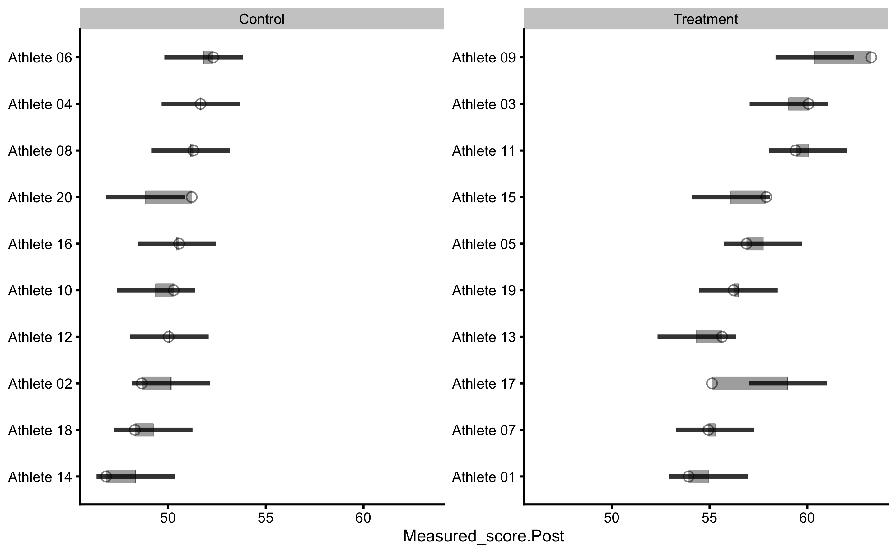
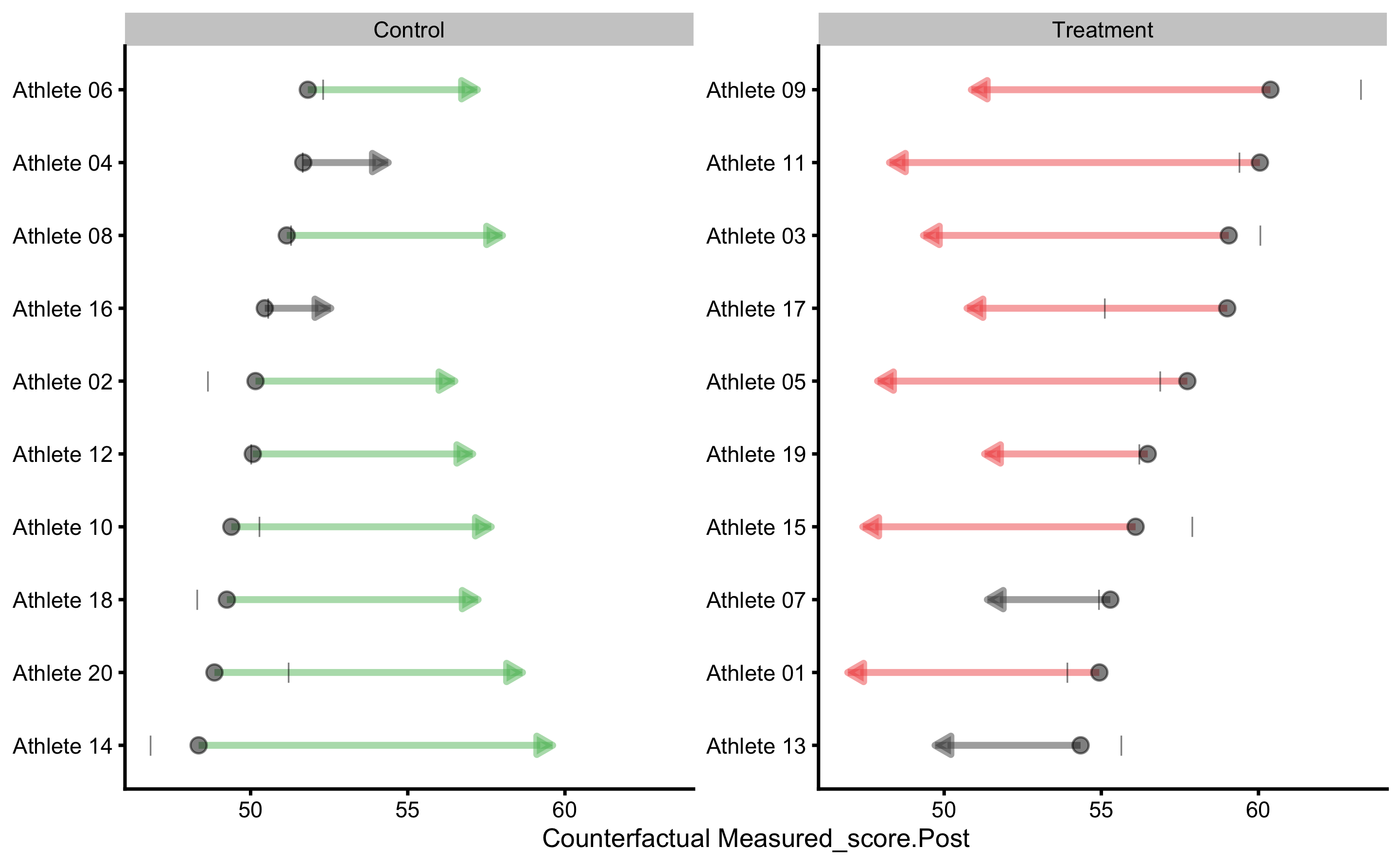
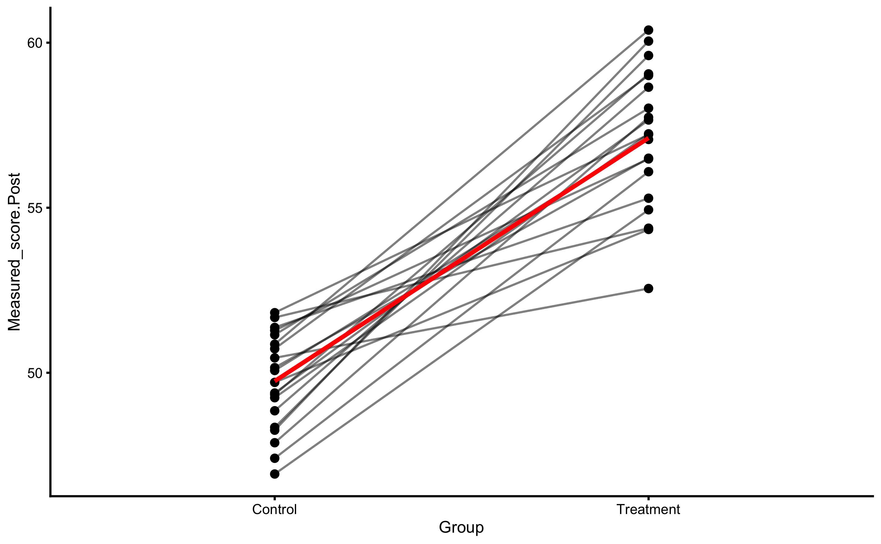
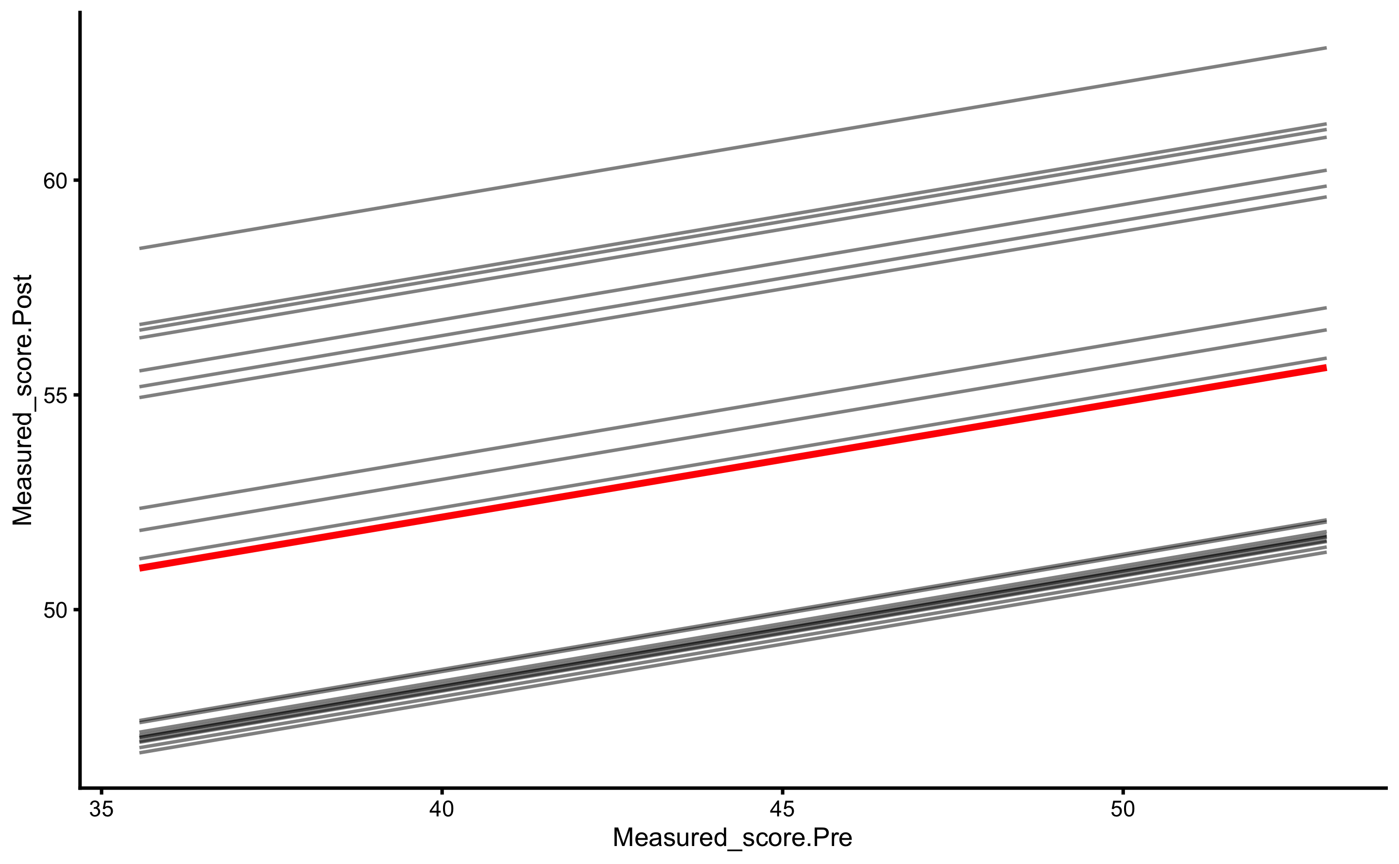
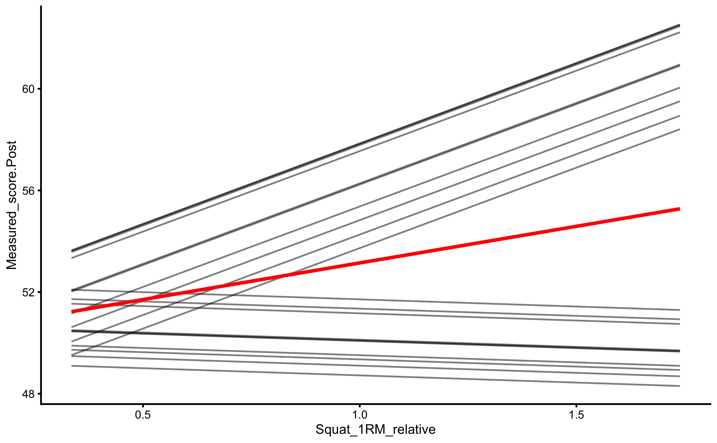
For the sake of comparisson between the models, let’s pull out estimated average, random, and variable treatment effects. Average treatment effect (pATE) is estimated using the mean of the pooled (absolute) counterfactual effects (see the previous model print summaries). Variable treatment effect (pVTE) is estimated using the SD of the pooled (absolute) counterfactual effects. Random treatment effect (RTE) is estimated using the group residuals as explained thorough this chapter.
model_estimates <- rbind(
  data.frame(
    model = "base",
    pATE = base_model$extra$average_treatment_effect,
    pVTE = base_model$extra$variable_treatment_effect,
    RTE =  base_model$extra$random_treatment_effect
  ),
  data.frame(
    model = "pre-test",
    pATE = pre_test_model$extra$average_treatment_effect,
    pVTE = pre_test_model$extra$variable_treatment_effect,
    RTE =  pre_test_model$extra$random_treatment_effect
  ),
  data.frame(
    model = "covariate",
    pATE = covariate_model$extra$average_treatment_effect,
    pVTE = covariate_model$extra$variable_treatment_effect,
    RTE =  covariate_model$extra$random_treatment_effect
  ),
    data.frame(
    model = "interaction",
    pATE = interaction_model$extra$average_treatment_effect,
    pVTE = interaction_model$extra$variable_treatment_effect,
    RTE =  interaction_model$extra$random_treatment_effect
  )
)

model_estimates
#>         model     pATE         pVTE      RTE
#> 1        base 7.221484 0.000000e+00 2.298433
#> 2    pre-test 7.599370 3.992905e-15 2.521028
#> 3   covariate 7.421514 4.890290e-15 1.599750
#> 4 interaction 7.366309 2.715167e+00 1.476142
Using counterfactual prediction, which is estimated by changing the group (and also group interaction with the squat 1RM), allows us to estimate average treatment effect (i.e. systematic or expected treatment effect) from the model with interactions.
Let’s plot the model predictive performance to compare the models. Let’s check the training performance (using training CV folds, where error bars represent min and max across training folds):
model_performace <- rbind(
  data.frame(
    model = "base",
    base_model$cross_validation$performance$summary$training
  ),
  data.frame(
    model = "pre-test",
    pre_test_model$cross_validation$performance$summary$training
  ),
  data.frame(
    model = "covariate",
    covariate_model$cross_validation$performance$summary$training
  ),
    data.frame(
    model = "interaction",
    interaction_model$cross_validation$performance$summary$training
  )
)

model_performace$model <- factor(
  model_performace$model,
  levels = rev(c("base", "pre-test", "covariate", "interaction"))
)

ggplot(
  model_performace,
  aes(y = model, x = mean)
) +
  theme_bw(8) +
  geom_errorbarh(aes(xmax = min, xmin = max),
    color = "black",
    height = 0
  ) +
  geom_point() +
  xlab("") +
  ylab("") +
  facet_wrap(~metric, scales = "free_x")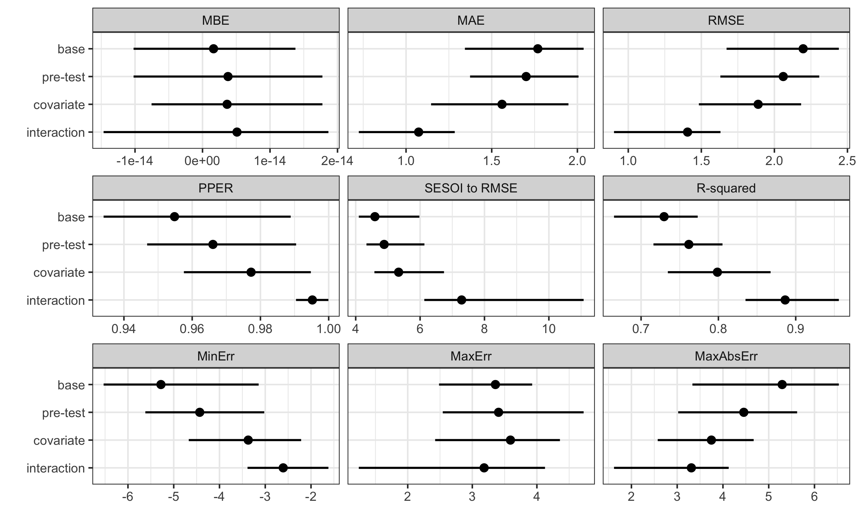
As can be seen from the figure, interaction model has the best training folds predictive performance. What about performance on the testing CV folds?
model_performace <- rbind(
  data.frame(
    model = "base",
    base_model$cross_validation$performance$summary$testing
  ),
  data.frame(
    model = "pre-test",
    pre_test_model$cross_validation$performance$summary$testing
  ),
  data.frame(
    model = "covariate",
    covariate_model$cross_validation$performance$summary$testing
  ),
    data.frame(
    model = "interaction",
    interaction_model$cross_validation$performance$summary$testing
  )
)

model_performace$model <- factor(
  model_performace$model,
  levels = rev(c("base", "pre-test", "covariate", "interaction"))
)

ggplot(
  model_performace,
  aes(y = model, x = mean)
) +
  theme_bw(8) +
  geom_errorbarh(aes(xmax = min, xmin = max),
    color = "black",
    height = 0
  ) +
  geom_point() +
  xlab("") +
  ylab("") +
  facet_wrap(~metric, scales = "free_x")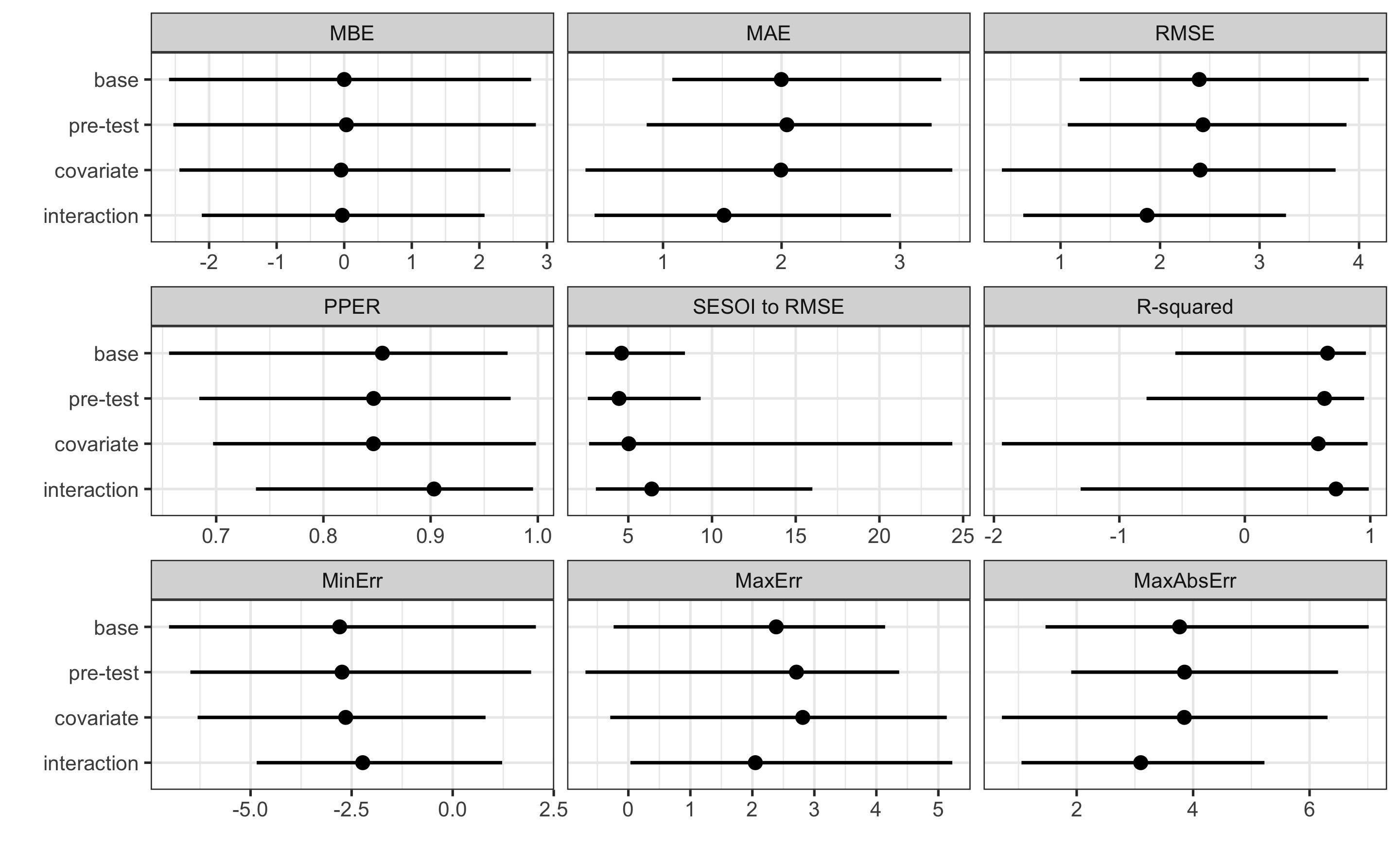
Interaction model is better, but not drastically better. Mean testing PPER is pretty good, over 0.9 indicating good practical predictive performance of this model.
Although the simple differences method or linear regression model helped us to explain overall treatment effects, predictive approach can tell us if we are able to predict individual responses, but also help in interpreting model counterfactually, particularly when there is interaction terms in the model.
We have used linear regression as out predictive model, but we could use any other model for that matter. Having RCT design allows us the interpret certain effect causally. Discussing these topics further is beyond the scope of this book (and the author) and the reader is directed to the references provided.