Chapter 8 Bootstrap
As already stated, some estimators have unknown sampling distribution, particularly those that might have more practical use and answer predictive questions by the practitioners (e.g. “what is the proportion of athletes I can expect to demonstrate beneficial response due to this treatment?”). Hence, the frequentist approach is very hard to use. With the Bayesian approach, some estimators might be really hard to be modeled and represented, researchers might be confused with the priors and likelihood function selections, there is knowledge needed to understand and diagnose sampling chains from MCMC algorithms and so forth.
Bootstrap comes for the rescue (30,40,43,79,159,160). Bootstrap is very simple and intuitive technique that is very easy to carry out. Let’s take an example to demonstrate simplicity of the bootstrap. Continuing with the height example, let’s assume that the following sample is collected for N=10 individuals: 167, 175, 175, 176, 177, 181, 188, 190, 197, 211cm. We are interested in estimating the true mean in the population, SD in the population, and proportion of individuals taller than 185cm (prop185; using algebraic method and estimated SD). The first step, as explained in the Description section of this book, is to estimate those parameters using sample. But how do we estimate the uncertainty around the sample estimates?
Bootstrap involves resampling from the sample itself and then recalculating estimates of interest. If we have N=10 observations in the collected sample, for each bootstrap resample we are going to draw 10x1 observations. Some observations might be drawn multiple times, while some might not be drawn at all. This is then repeated numerous times, e.g., 2,000-10,000 times and for each bootstrap resample the estimators of interest are estimated. Table 8.1 contains 10 bootstrap resamples with calculated estimators of interest. Bootstrap resample of number 0 represents the original sample.
| Boot resample | Observations | mean | SD | prop185 |
|---|---|---|---|---|
| 0 | 167 175 175 176 177 181 188 190 197 211 | 183.7 | 13.00 | 0.46 |
| 1 | 167 167 167 177 188 188 188 188 197 197 | 182.4 | 11.98 | 0.41 |
| 2 | 175 175 175 181 181 181 181 190 197 197 | 183.3 | 8.49 | 0.42 |
| 3 | 175 175 177 177 181 181 188 188 188 190 | 182.0 | 5.98 | 0.31 |
| 4 | 167 181 181 181 181 188 188 197 197 197 | 185.8 | 9.61 | 0.53 |
| 5 | 167 176 176 177 181 188 190 190 211 211 | 186.7 | 14.71 | 0.55 |
| 6 | 167 167 167 175 177 177 188 188 190 211 | 180.7 | 13.88 | 0.38 |
| 7 | 175 175 175 176 177 177 181 181 188 190 | 179.5 | 5.50 | 0.16 |
| 8 | 175 175 175 176 177 181 188 190 190 190 | 181.7 | 6.96 | 0.32 |
| 9 | 176 176 177 181 190 190 190 190 197 211 | 187.8 | 10.97 | 0.60 |
| 10 | 167 167 175 175 175 176 176 177 177 188 | 175.3 | 5.83 | 0.05 |
| 11 | 175 177 181 181 181 188 190 197 197 211 | 187.8 | 11.21 | 0.60 |
| 12 | 175 175 175 176 176 177 181 188 190 211 | 182.4 | 11.47 | 0.41 |
| 13 | 175 175 177 181 181 188 190 190 211 211 | 187.9 | 13.43 | 0.59 |
| 14 | 167 175 175 176 177 177 188 190 211 211 | 184.7 | 15.34 | 0.49 |
| 15 | 175 177 177 181 181 188 188 190 211 211 | 187.9 | 13.21 | 0.59 |
| 16 | 167 175 175 175 177 177 181 188 190 197 | 180.2 | 8.92 | 0.30 |
| 17 | 175 175 175 176 177 177 181 190 190 197 | 181.3 | 8.04 | 0.32 |
| 18 | 167 175 175 175 176 177 177 188 188 188 | 178.6 | 7.07 | 0.18 |
| 19 | 167 167 175 177 181 188 190 197 197 211 | 185.0 | 14.24 | 0.50 |
| 20 | 167 167 175 175 176 176 177 181 197 211 | 180.2 | 13.66 | 0.36 |
If we repeat this procedure 10,000 times, we can visualize bootstrap distribution of the estimators (Figure 8.1).
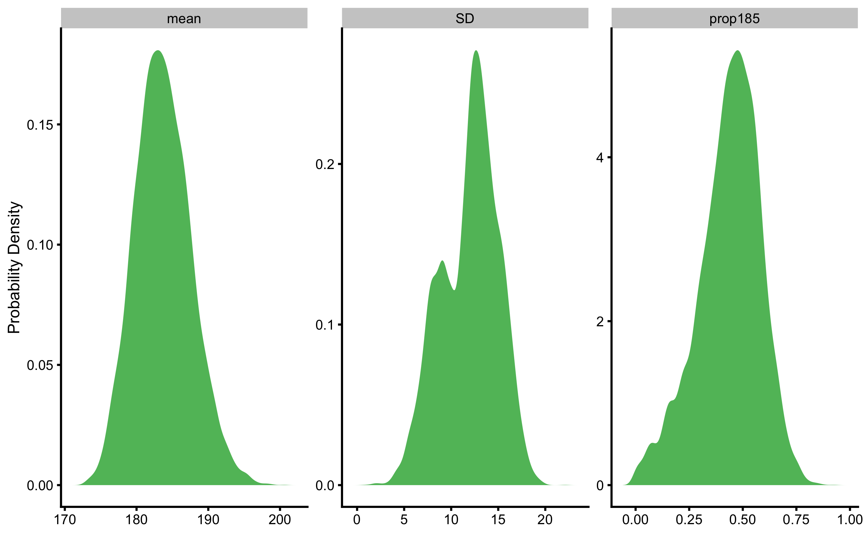
Figure 8.1: Bootstrap distribution of the estimators using 10,000 resamples
How should this bootstrap distribution be interpreted? In “Elements of Statistical Learning”, the following quote regarding bootstrap distribution can be found (65):
“In this sense, the bootstrap distribution represents an (approximate) nonparametric, noninformative posterior distribution for our parameter. But this bootstrap distribution is obtained painlessly — without having to formally specify a prior and without having to sample from the posterior distribution. Hence we might think of the bootstrap distribution as a “poor man’s” Bayes posterior. By perturbing the data, the bootstrap approximates the Bayesian effect of perturbing the parameters, and is typically much simpler to carry out"
Although the bootstrap was originally developed as a purely frequentist device (42), as per the quote above, it can be treated as “poor man’s” Bayes posterior.
8.1 Summarizing bootstrap distribution
Bootstrap allows for both estimation and hypothesis testing. When it comes to estimations, point estimate of the bootstrap distribution is the sample parameter estimate. Confidence intervals around sample estimate are usually calculated using percentile approach (or ETI), or other approaches such as adjusted bootstrap percentile (BCa) (30,40,43,79,159,160), or even HDI as used with Bayesian posterior distributions. In this book I will utilize BCa intervals unless otherwise stated.
Hypothesis testing using the bootstrap distribution is possible through calculated p-value (159,160). This not only allows for bootstrap NHST, but also all other MET, as well as MBI estimates (which assumes Bayesian interpretation of the bootstrap distributions). This is simply done by counting bootstrap sample estimates that are below or above particular threshold (i.e. null-hypothesis or SESOI). The R code (153,162) below demonstrates how two-way NHST can be performed as well as probability of lower, equivalent, and higher effect given the SESOI thresholds.
null_hypothesis <- 0 # Value for the null

SESOI_lower <- -1 # threshold for the 'lower' effect magnitude
SESOI_upper <- 1 # threshold for the 'upper' effect magnitude

# Calculation of the p-value
# where boot.estimator is the boostrap resample values for the estimator
# of interest
p_value <- mean(boot.estimator > null_hypothesis)
p_value <- p_value + 0.5 * mean(boot.estimator == null_hypothesis)
p_value <- 2 * min(c(p_value, 1 - p_value)) # Two-way p-value

# Calculate probability of lower, equivalent and higher effect magnitude
lower <- mean(boot.estimator < SESOI_lower)
higher <- mean(boot.estimator > SESOI_upper)
equivalent <- 1 - (lower + higher)
8.2 Bootstrap Type I errors
As we already did with the frequentist and Bayesian inference, let’s get estimates of Type I errors for bootstrap method (10,000 bootstrap resamples) by drawing 1,000 samples of N=20 observations from the population where the true mean height is equal to 177.8cm and SD is equal to 10.16cm. Besides estimating Type I error for the sample mean, we can also estimate Type I errors for sample SD and prop185, since the true population values are known. In the case of prop185, the true population value is equal to 0.24. Type I error is committed when the the 95% bootstrap CIs of the sample estimate don’t cross the true value in the population. Figure 8.2 depicts the first 100 samples out of the total of 1,000, taken from the population with calculated 95% bootstrap CIs. CIs that missed the true population parameter value are depicted in red. Table 8.2 contains the summary for this simulation.
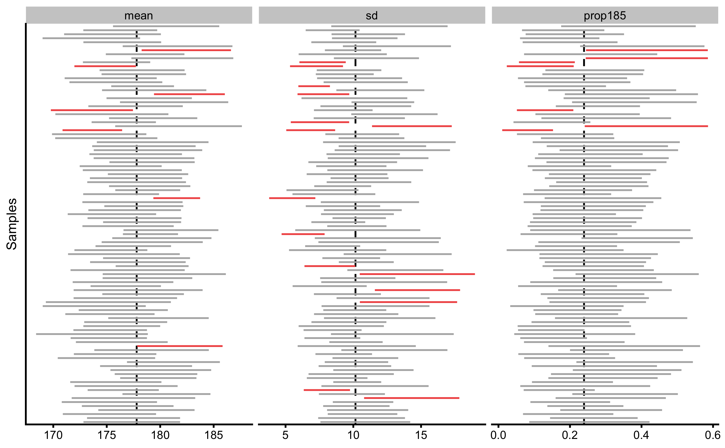
Figure 8.2: Bootstrap \(95\%\)confidence intervals. Intervals not capturing the true population parameter are colored in red
| parameter | Sample | Correct % | Type I Errors % |
|---|---|---|---|
| mean | 1000 | 92.7 | 7.3 |
| sd | 1000 | 89.9 | 10.1 |
| prop185 | 1000 | 93.1 | 6.9 |
As can be seen from the Table 8.2, Type I error for the \(\sigma\) parameter is larger than expected. This could be due to the non-symmetrical bootstrap distribution that might not be perfectly represented with the BCa approach of calculating CIs.
I am not hiding my preference for the bootstrap methods due to their intuitive nature and simple usage for generating inferences for any estimator.
However, bootstrap is not panacea and there are caveats especially for the small samples sizes (159,160,198,200).
References
30. Canty, A and Ripley, BD. Boot: Bootstrap R (S-Plus) Functions. 2017.
40. Davison, AC and Hinkley, DV. Bootstrap Methods and Their Applications. Cambridge: Cambridge University Press, 1997.
42. Efron, B. Bayesians, Frequentists, and Scientists. Journal of the American Statistical Association 100: 1–5, 2005.
43. Efron, B and Hastie, T. Computer Age Statistical Inference: Algorithms, Evidence, and Data Science. 1 edition. New York, NY: Cambridge University Press, 2016.
65. Hastie, T, Tibshirani, R, and Friedman, JH. The elements of statistical learning: Data mining, inference, and prediction. 2nd ed. New York, NY: Springer, 2009.
79. Hesterberg, TC. What Teachers Should Know About the Bootstrap: Resampling in the Undergraduate Statistics Curriculum. The American Statistician 69: 371–386, 2015.
153. R Core Team. R: A Language and Environment for Statistical Computing. Vienna, Austria: R Foundation for Statistical Computing, 2018.
159. Rousselet, GA, Pernet, CR, and Wilcox, RR. A practical introduction to the bootstrap: A versatile method to make inferences by using data-driven simulations., 2019.
162. RStudio Team. RStudio: Integrated Development Environment for R. Boston, MA: RStudio, Inc., 2016.
198. Wilcox, R, Peterson, TJ, and McNitt-Gray, JL. Data Analyses When Sample Sizes Are Small: Modern Advances for Dealing With Outliers, Skewed Distributions, and Heteroscedasticity. Journal of Applied Biomechanics 34: 258–261, 2018.
200. Wilcox, RR and Rousselet, GA. A guide to robust statistical methods in neuroscience. bioRxiv, 2017.