Chapter 7 Bayesian perspective

Bayesian inference is reallocation of plausibility (credibility) across possibilities (107,108,130). Kruschke and Liddell (107) wrote in their paper as follows:

“The main idea of Bayesian analysis is simple and intuitive. There are some data to be explained, and we have a set of candidate explanations. Before knowing the new data, the candidate explanations have some prior credibility of being the best explanation. Then, when given the new data, we shift credibility toward the candidate explanations that better account for the data, and we shift credibility away from the candidate explanations that do not account well for the data. A mathematically compelling way to reallocate credibility is called Bayes’ rule. The rest is just details.”

The aim of this section is to provide the gross overview of the Bayesian inference using grid approximation method (130), which is excellent teaching tool, but very limited for Bayesian analysis beyond simple mean and simple linear regression inference. More elaborate discussion on the Bayesian methods, such as Bayes factor, priors selection, model comparison, and Markov Chain Monte Carlo sampling is beyond the scope of this book. Interested readers are directed to the references provided and suggested readings at the end of this book.

7.1 Grid approximation

To showcase the rationale behind Bayesian inference let’s consider the same example used in Frequentist perspective chapter - the male height. The question we are asking is, given our data, what is the true average male height (mean; mu or Greek letter $\mu$) and SD (sigma or Greek letter $\sigma$). You can immediately notice the difference in the question asked. In the frequentist approach we are asking “What is the probability of observing the data³¹ (estimator, like mean or Cohen's d), given the null hypothesis?”

True average male height and true SD represents parameters, and with Bayesian inference we want to relocate credibility across possibilities of those parameters (given the data collected). For the sake of this simplistic example, let’s consider the following possibilities for the mean height: 170, 175, 180cm, and for SD: 9, 10, 11cm. This gives us the following grid (Table 7.1), which combines all possibilities in the parameters, hence the name grid approximation. Since we have three possibilities for each parameter, the grid consists of 9 total possibilities.

Table 7.1: **Parameter possibilities**
mu	sigma
170	9
175	9
180	9
170	10
175	10
180	10
170	11
175	11
180	11

7.2 Priors

Before analyzing the collected data sample, with Bayesian inference we want to state the prior beliefs in parameter possibilities. For example, I might state that from previous data collected, I believe that the mean height is around 170 and 180cm, with a peak at 175cm (e.g. approximating normal curve). We will come back to topic of prior later on, but for now lets use uniform or vague prior, which assigns equal plausibility to all mean height and SD possibilities. Since each parameter has three possibilities, and since probabilities needs to sum up to 1, each possibility has probability of 1/3 or 0.333. This is assigned to our grid in the Table 7.2.

Table 7.2: **Parameter possibilities with priors**
mu	sigma	mu prior	sigma prior
170	9	0.33	0.33
175	9	0.33	0.33
180	9	0.33	0.33
170	10	0.33	0.33
175	10	0.33	0.33
180	10	0.33	0.33
170	11	0.33	0.33
175	11	0.33	0.33
180	11	0.33	0.33

7.3 Likelihood function

The sample height data we have collected for N=5 individuals is 167, 192, 183, 175, 177cm. From this sample we are interested in making inference to the true parameter values (i.e. mean and SD, or $\mu$ and $\sigma$). Without going into the Bayes theorem for inverse probability, the next major step is the likelihood function. Likelihood function gives us a likelihood of observing data, given parameters. Since we have 9 parameter possibilities, we are interested in calculating the likelihood of observing the data for each possibility. This is represented with a following Equation (7.1):

\[\begin{equation} L(x|\mu, \sigma) = \prod_{i=1}^{n}f(x_{i}, \mu, \sigma) \tag{7.1} \end{equation}\]

The likelihood of observing the data is calculated by taking the product (indicated by $\prod_{i=1}^{n}$ sign in the Equation (7.1) of likelihood of observing individual scores. The likelihood function is normal probability density function (PDF)³²:, whose parameters are $\mu$ and $\sigma$ (see Figure 7.1). This function has the following Equation (7.2):

\[\begin{equation} f(x_{i}, \mu, \sigma) = \frac{e^{-(x - \mu)^{2}/(2\sigma^{2}) }} {\sigma\sqrt{2\pi}} \tag{7.2} \end{equation}\]

Let’s take a particular possibility of $\mu$ and $\sigma$, e.g. 175cm and 9cm, and calculate likelihoods for each observed score (Table 7.3).

Table 7.3: **Likelihoods of observing scores given $\mu$ and $\sigma$ equal to 175cm and 9cm**
mu	sigma	x	likelihood
175	9	167	0.03
175	9	192	0.01
175	9	183	0.03
175	9	175	0.04
175	9	177	0.04

Now, to estimate likelihood of the sample, we need to take the product of each individual score likelihoods. However, now we have a problem, since the result will be very, very small number (1.272648^{-8}). To solve this issue, we take the log of the likelihood function. This is called log likelihood (LL) and it is easier to compute without the fear of losing digits. Table 7.4 contains calculated log from the score likelihood.

Table 7.4: **Likelihoods and log likelihoods of observing scores given $\mu$ and $\sigma$ equal to 175cm and 9cm**
mu	sigma	x	likelihood	LL
175	9	167	0.03	-3.51
175	9	192	0.01	-4.90
175	9	183	0.03	-3.51
175	9	175	0.04	-3.12
175	9	177	0.04	-3.14

Rather than taking a product of the LL to calculate the overall likelihood of the sample, we take the sum. This is due the properties of the logarithmic algebra, where $\log{x_1\times x_2} = log{x_1} + log{x_2}$, which means that if we take the exponent of the sum of the log likelihoods, we will get the same result as taking the exponent of the product of likelihoods. Thus the overall log likelihood of observing the sample is equal to -18.18. If we take the exponent of this, we will get the same results as the product of individual likelihoods, which is equal to 1.272648^{-8}. This mathematical trick is needed to prevent very small numbers and thus loosing precision.

If we repeat the same procedure for every parameter possibility in our grid, we get the following log likelihoods (Table 7.5). This procedure is also visually represented in the Figure 7.1 for easier comprehension.

Table 7.5: **Sum of data log likelihoods for parameter possibilities**
mu	sigma	mu prior	sigma prior	LL
170	9	0.33	0.33	-20.12
175	9	0.33	0.33	-18.18
180	9	0.33	0.33	-17.78
170	10	0.33	0.33	-19.79
175	10	0.33	0.33	-18.21
180	10	0.33	0.33	-17.89
170	11	0.33	0.33	-19.63
175	11	0.33	0.33	-18.32
180	11	0.33	0.33	-18.06

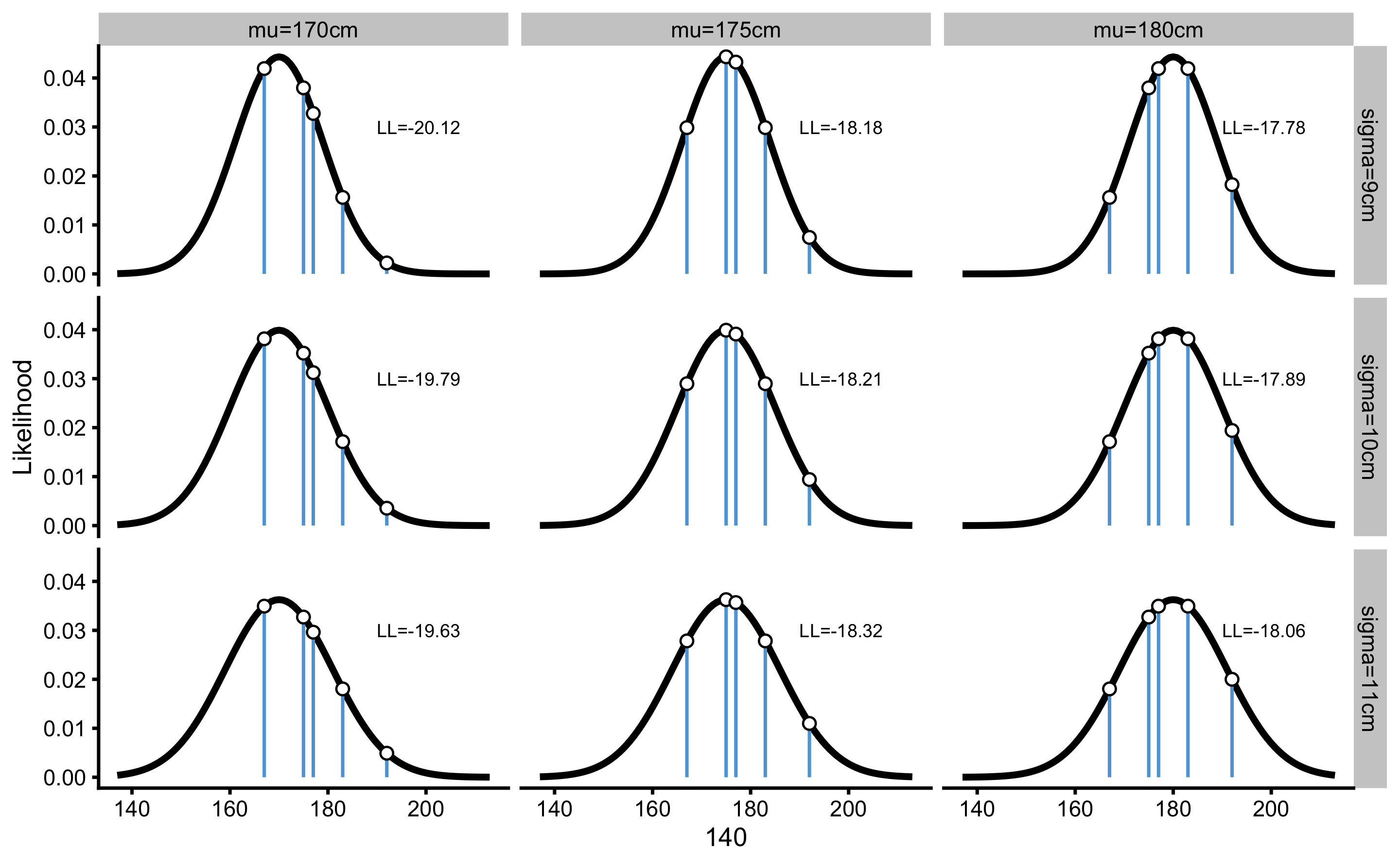
$Likelihood of data given parameters. $\mu$ and $\sigma$ represent parameters for which we want to estimate likelihood of observing data collected$

Figure 7.1: Likelihood of data given parameters. $\mu$ and $\sigma$ represent parameters for which we want to estimate likelihood of observing data collected

7.4 Posterior probability

To get the posterior probabilities of parameter possibilities, likelihoods need to be multiplied with priors ($posterior = prior \times likelihood$). This is called Bayesian updating. Since we have log likelihoods, we need to sum the log likelihoods with log of priors instead ($\log{posterior} = \log{prior} + \log{likelihood}$). To get the posterior probability, after converting log posterior to posterior using exponent ($posterior = e^{\log{posterior}}$)³³, we need to make sure that probabilities of parameter possibility sum to one. This is done by simply dividing probabilities for each parameter possibility by the sum of probabilities.

Table 7.6 contains the results of Bayesian inference. The posterior probabilities are called joint probabilities since they represent probability of a combination of particular $\mu$ and $\sigma$ possibility.

Table 7.6: **Estimated posterior probabilities for parameter possibilities given the data**
mu	sigma	mu prior	sigma prior	LL	posterior
170	9	0.33	0.33	-20.12	0.02
175	9	0.33	0.33	-18.18	0.14
180	9	0.33	0.33	-17.78	0.20
170	10	0.33	0.33	-19.79	0.03
175	10	0.33	0.33	-18.21	0.13
180	10	0.33	0.33	-17.89	0.18
170	11	0.33	0.33	-19.63	0.03
175	11	0.33	0.33	-18.32	0.12
180	11	0.33	0.33	-18.06	0.15

Table 7.6 can be be converted into 3x3 matrix, with possibilities of $\mu$ in the columns, and possibilities of the $\sigma$ in the rows and posterior joint probabilities in the cells (Table 7.7). The sums of the joint probabilities in the Table 7.7 margins represent marginal probabilities for parameters.

Table 7.7: **Joint distribution of the parameter possibilities.** Sums at the table margins represent marginal probabilities
	170	175	180	Sum
9	0.02	0.14	0.20	0.36
10	0.03	0.13	0.18	0.34
11	0.03	0.12	0.15	0.30
Sum	0.08	0.38	0.54	1.00

Since we have only two parameters, the joint probabilities can be represented with the heat map. Figure 7.2 is a visual representation of the Table 7.7.

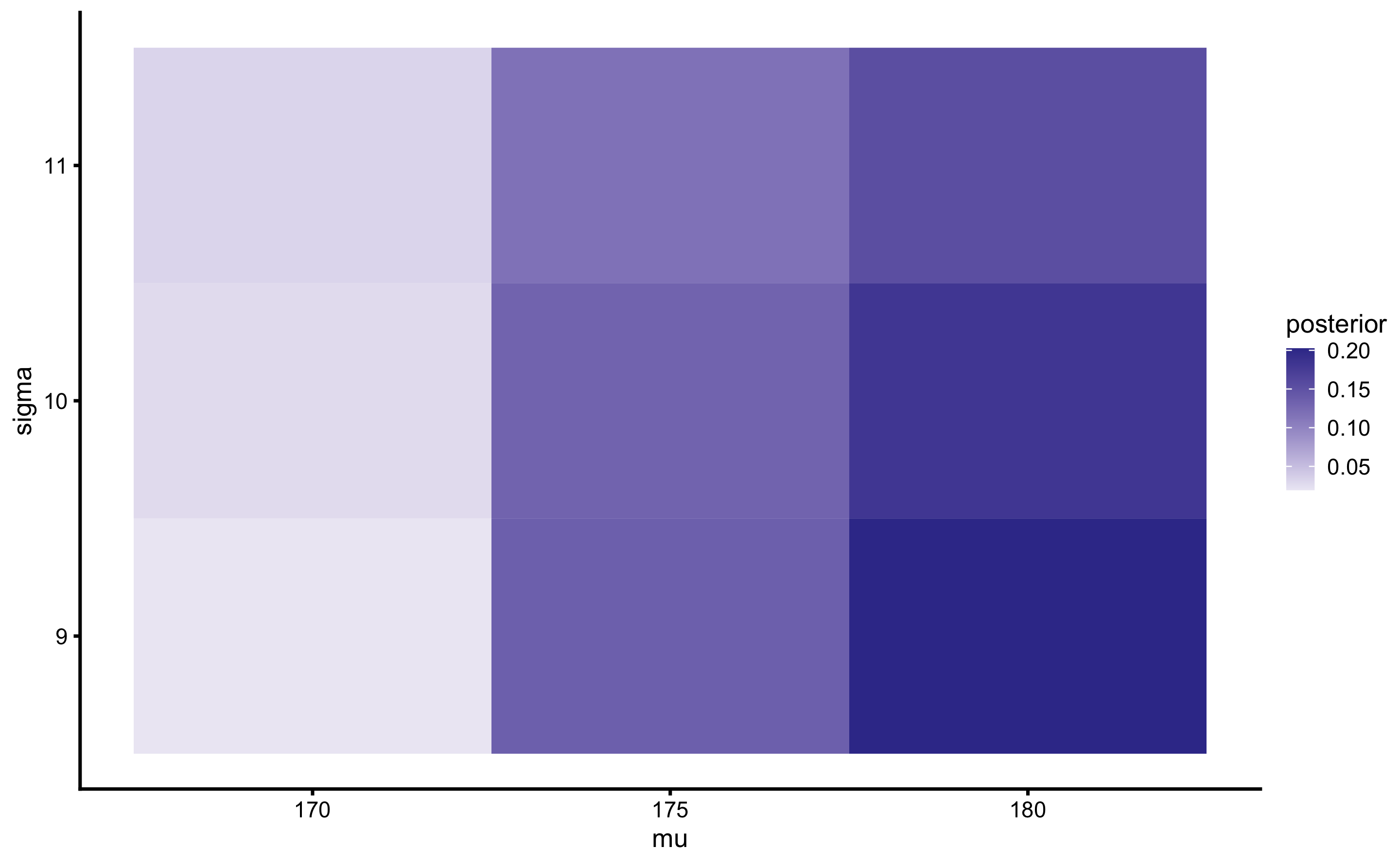
$Heat map of $\mu$ and $\sigma$ joint probabilities$

Figure 7.2: Heat map of $\mu$ and $\sigma$ joint probabilities

When we have more than 2 parameters, visualization of joint probabilities get’s tricky and we rely on visualizing marginal posterior probabilities of each parameter instead. As explained, marginal probabilities are calculated by summing all joint probabilities for a particular parameter possibility (see Table 7.7). Figure @ref(fig:(marginal-prior-posterior) depicts marginal probabilities (including prior probabilities) for $\mu$ and $\sigma$.

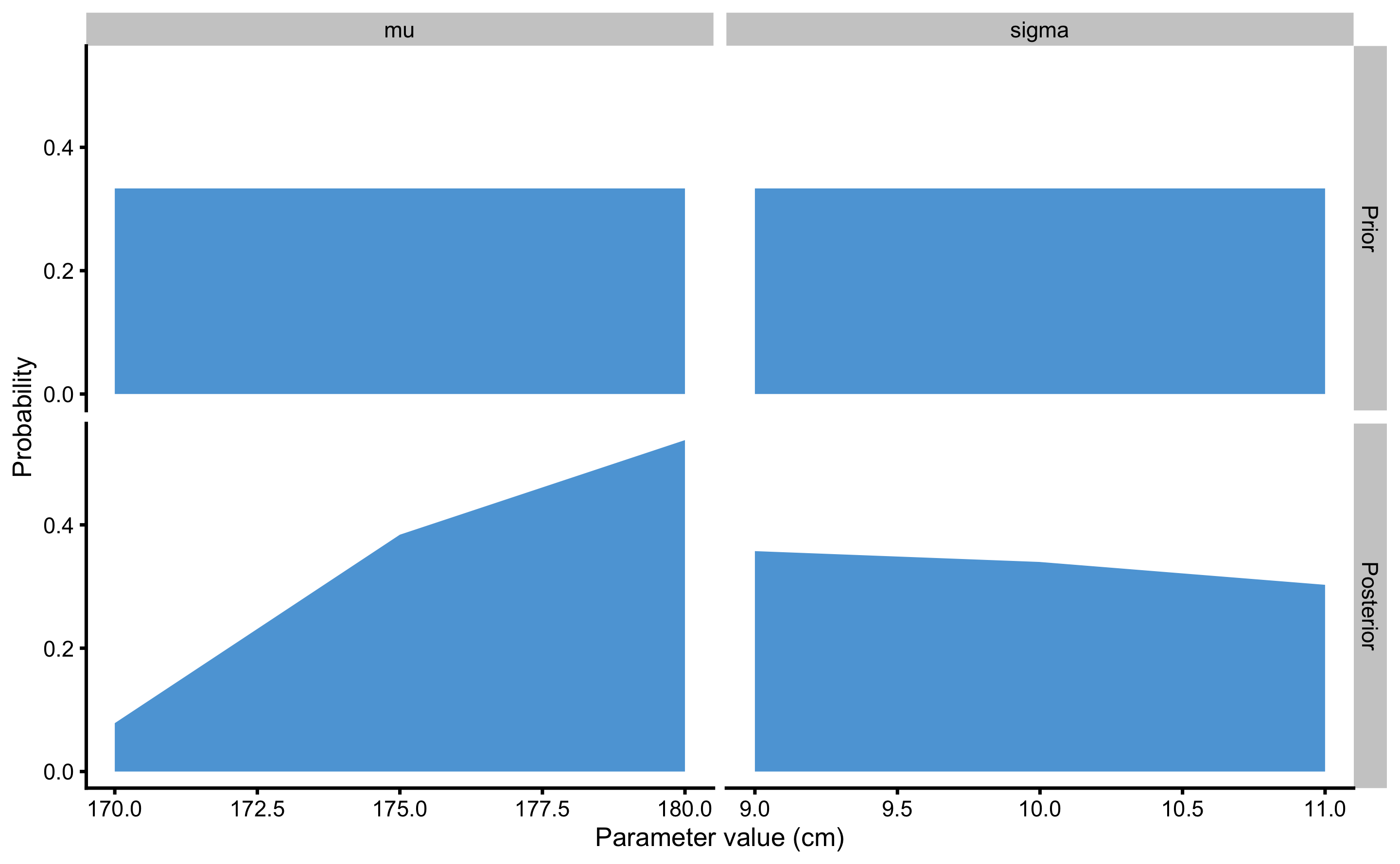
Figure 7.3: Prior and posterior distributions resulting from simplified grid-approximation example

As can be seen from the Figures 7.2 and 7.3, the most likely parameter possibilities, given the data, are $\mu$ of 180cm and $\sigma$ of 9cm.

7.5 Adding more possibilities

So far, we have made this very granular in order to be understood. However, since we are dealing with continuous parameters, performing grid approximation for more than 9 total parameter possibilities seems warranted. The calculus is exactly the same, as well as the sample collected, but now we will use the larger range for both $\mu$ (160-200cm) and $\sigma$ (1-30cm), each with 100 possibilities. We are estimating credibility for total of $100 \times 100 = 10,000$ parameter possibilities. Figure 7.4 depicts heat map for the joint probabilities, and Figure 7.5 depicts prior and posterior marginal distributions for each parameter.

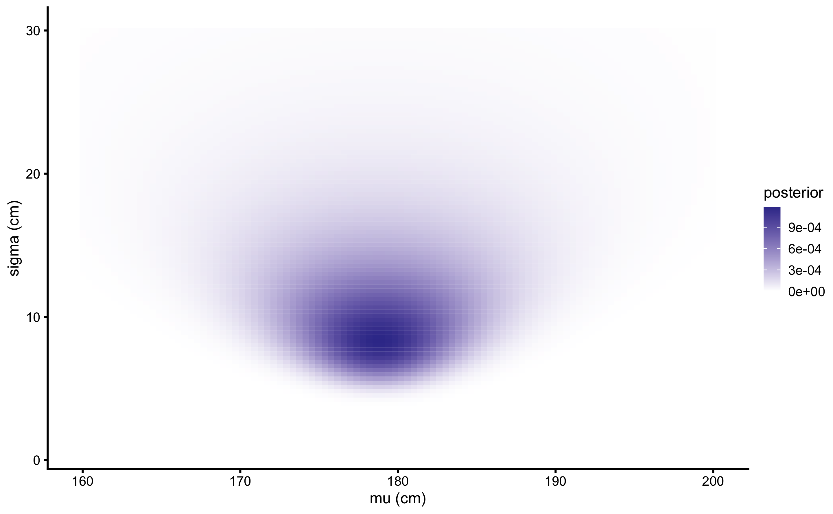
$Heat map of $\mu$ and $\sigma$ joint probabilities when $100\times 100$ grid-approximation is used$

Figure 7.4: Heat map of $\mu$ and $\sigma$ joint probabilities when $100\times 100$ grid-approximation is used

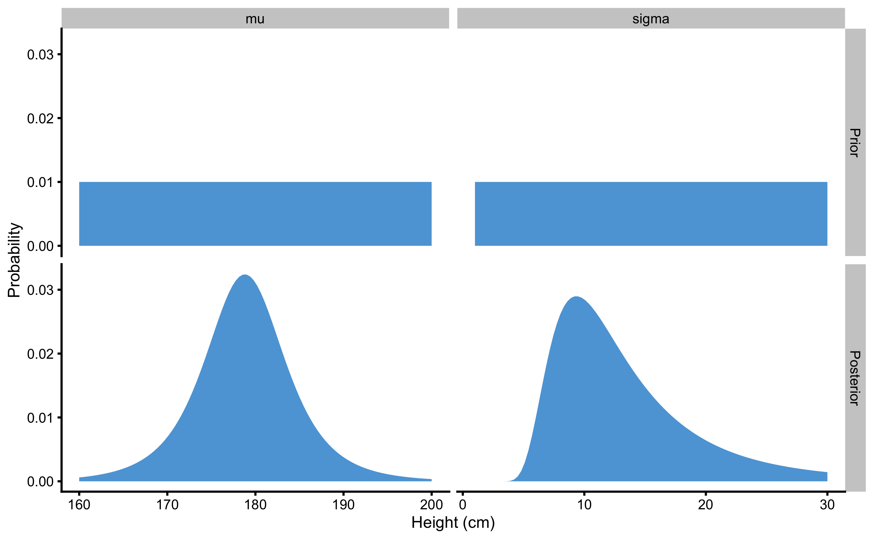
$Prior and posterior distributions resulting from $100\times 100$ grid-approximation example$

Figure 7.5: Prior and posterior distributions resulting from $100\times 100$ grid-approximation example

Grid approximation utilized here is great for educational purposes and very simple models, but as number of parameters increases, the number of total parameter possibility grow so large, that it might take millions of years for a single computer to compute the posterior distributions. For example, if we have linear regression model with two predictors, we will have 4 parameters to estimate (intercept $\beta_{0}$, predictor one $\beta_{1}$, predictor two $\beta_{2}$, and residual standard error $\sigma$), and if we use 100 possibilities for each parameter, we will get 10^8 total number of possibilities.

This was the reason why Bayesian inference was not very practical. Until algorithms such as Markov Chain Monte Carlo (MCMC) emerged making Bayesian inference a walk in the park. Statistical Rethinking book by Richard McElreath is outstanding introduction into these topics.

7.6 Different prior

In this example we have used vague priors for both $\mu$ and $\sigma$. But let’s see what happens when I strongly believe (before seeing the data), that $\mu$ is around 190cm (using normal distribution with mean 190 and SD of 2 to represent this prior), but I do not have a clue about $\sigma$ prior distribution and I choose to continue using uniform prior for this parameter.

This prior belief is, of course, wrong, but maybe I am biased since I originate, let’s say from Montenegro, country with one of the tallest men. Figure 7.6 contains plotted prior and posterior distributions. As can be seen, using very strong prior for $\mu$ shifted the posterior distribution to the higher heights. In other words, the data collected were not enough to overcome my prior belief about average height.

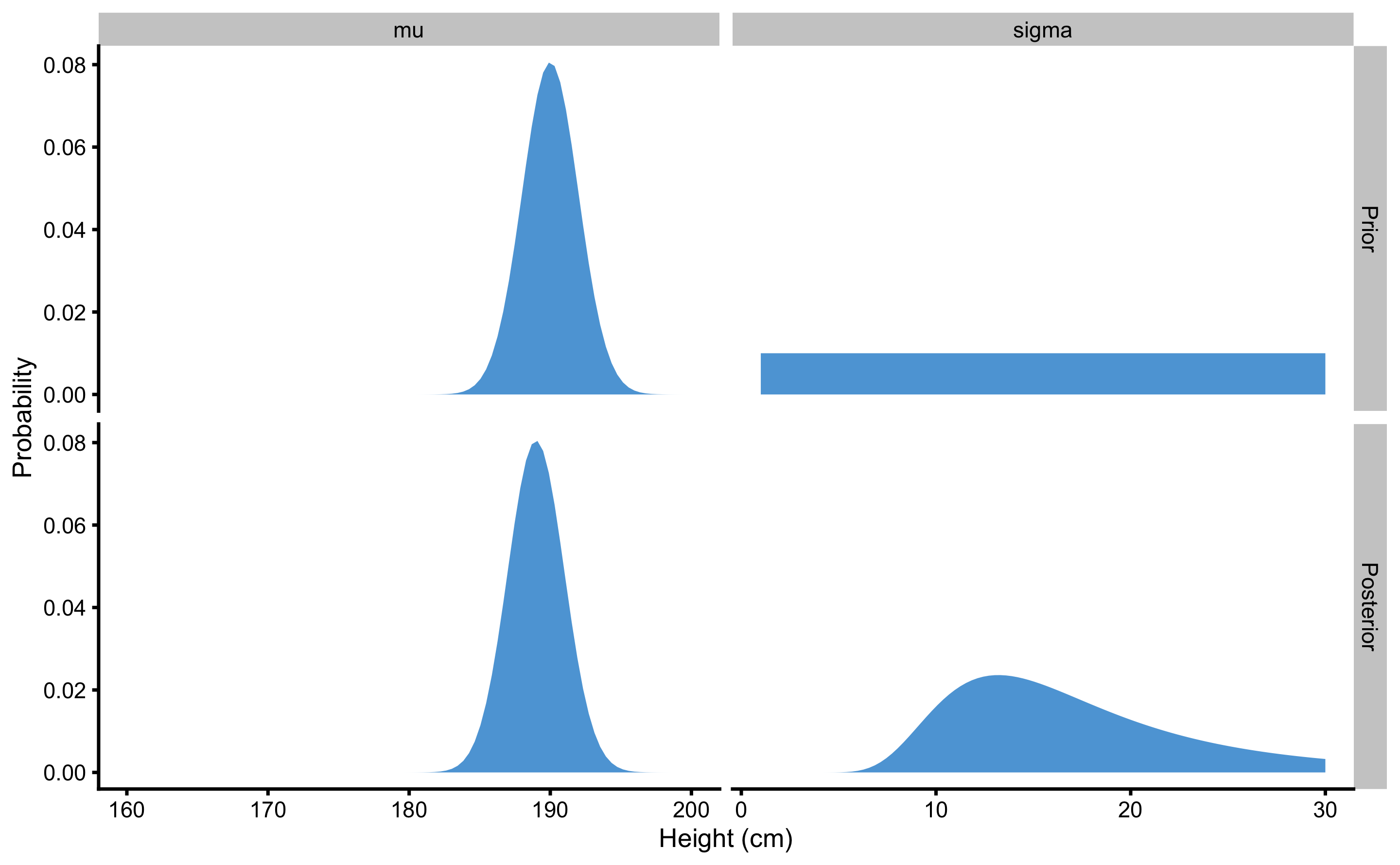
Figure 7.6: Effects of very strong prior on posterior

7.7 More data

The sample height data we have collected for N=5 individuals (167, 192, 183, 175, 177cm) was not strong to overcome prior belief. However, what if we sampled N=100 males from known population of known mean height of 177.8 and SD of 10.16? Figure 7.7 depicts prior and posterior distributions in this example. As can be seen, besides having narrower posterior distributions for $\mu$ and $\sigma$, more data was able to overcome my strong prior bias towards mean height of 190cm.

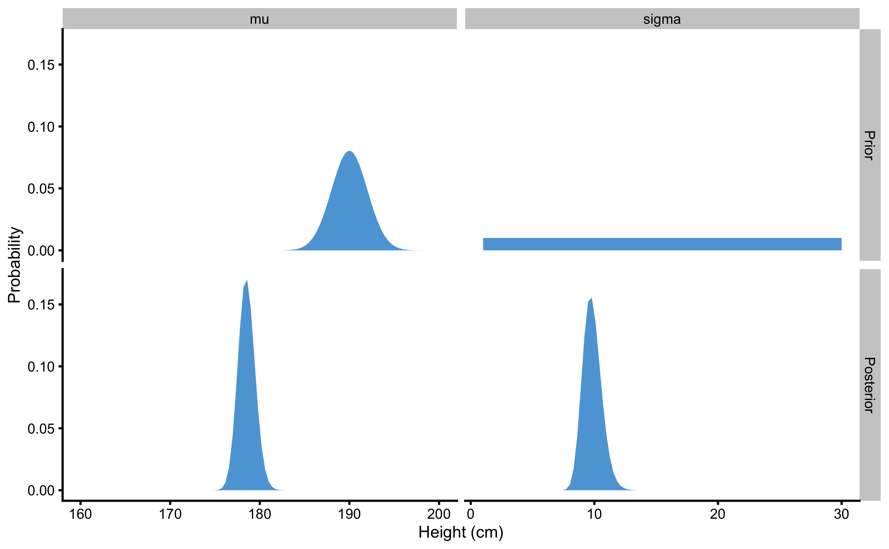
Figure 7.7: When larger sample is taken (N=100) as opposed to smaller sample (N=20), strong prior was not able to influence the posterior distribution

7.8 Summarizing prior and posterior distributions with MAP and HDI

In Bayesian statistics, the prior and posterior distributions are usually summarized using highest maximum a posteriori (MAP) and 90% or 95% highest density interval (HDI) (107,108,130). MAP is simply a mode, or the most probable point estimate. In other words, a point in the distribution with the highest probability. With normal distribution, MAP, mean and median are identical. The problems arise with distributions that are not symmetrical.

HDI is similar to frequentist CI, but represents an interval which contains all points within the interval that have higher probability density than points outside the interval (126,129). HDI is more computationally expensive to estimate, but compared to equal-tailed interval (ETI) or percentile interval, that typically excludes 2.5% or 5% from each tail of the distribution (for 95% or 90% confidence respectively), HDI is not equal-tailed and therefore always includes the mode(s) of posterior distributions (126,129).

Figure 7.8 depicts comparison between MAP and 90% HDI, median and 90% percentile interval or ETI, and mean and $\pm1.64 \times SD$ for 90% confidence interval. As can be seen from the Figure 7.8, the distribution summaries differ since the distribution is asymmetrical and not-normal. Thus, in order to summarize prior or posterior distribution, MAP and HDI are most often used, apart from visual representation.

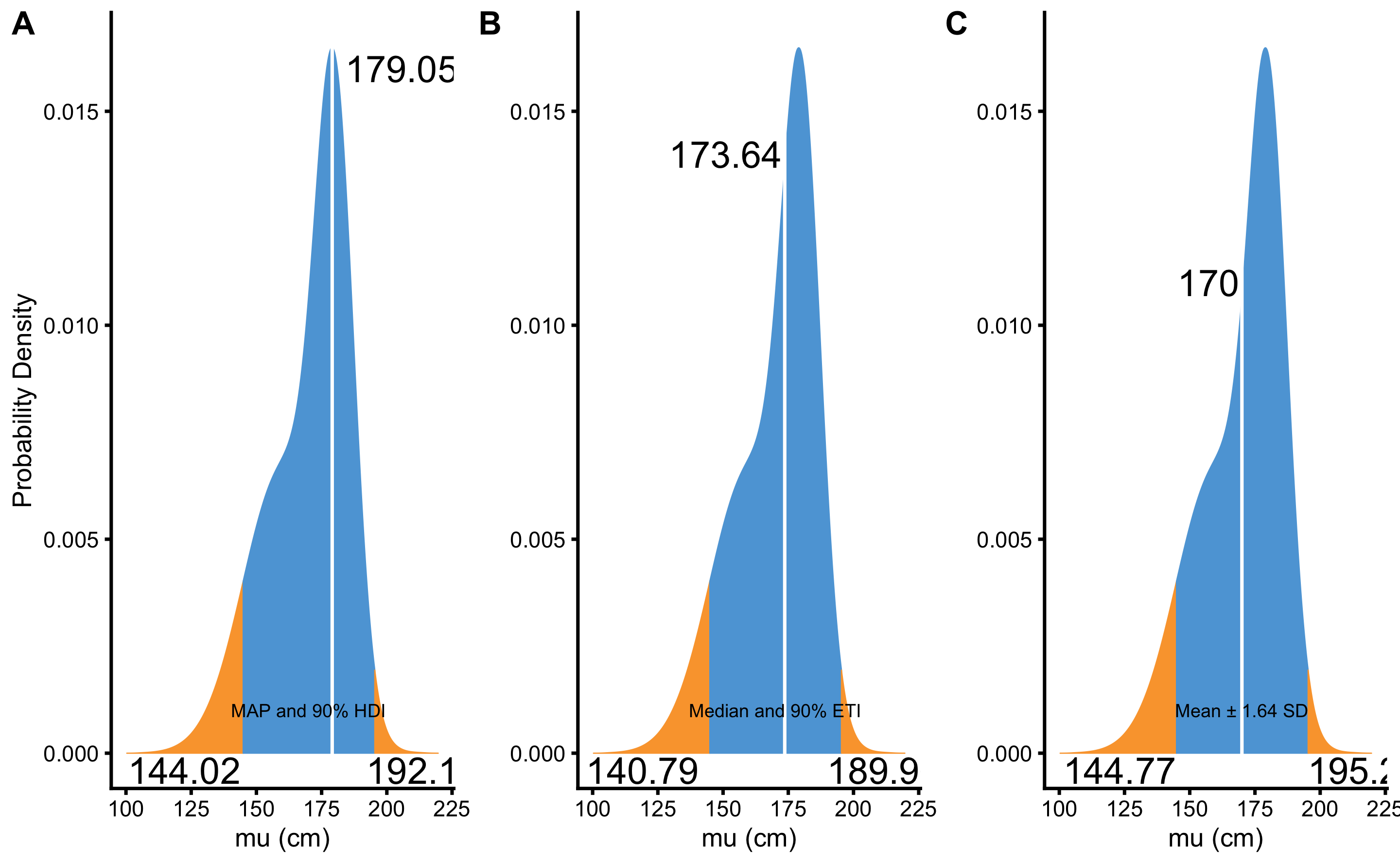
$Summarizing prior and posterior distribution. A. MAP and $90\%$ HDI. B. Median and $90\%$ ETI. C. Mean and $\pm1.64\times SD$$

Figure 7.8: Summarizing prior and posterior distribution. A. MAP and $90\%$ HDI. B. Median and $90\%$ ETI. C. Mean and $\pm1.64\times SD$

Using SESOI as a trivial range, or as a ROPE (107,108), Bayesian equivalence test can be performed by quantifying proportion of posterior distribution inside the SESOI band (107,108,126,127). Magnitude Based Inference discussed in the the previous chapter, would also be valid way of describing the posterior distribution.

Besides estimating using MAP and HDI, Bayesian analysis also allows hypothesis testing using Bayes factor or MAP based p-value (107,108,126,127). Discussing these concepts is out of the range of this book and interested readers can refer to references provided for more information.

7.9 Comparison to NHST Type I errors

How do the Bayesian HDIs compare to frequentist CIs? What are the Type I error rates when the data is sampled from the null-hypothesis? To explore this question, I will repeat the simulation from New Statistics: Confidence Intervals and Estimation section, where 1,000 samples of N=20 observations are sampled from a population where the true mean height is equal to 177.8cm and SD is equal to 10.16cm. Type I error is committed when the the 95% CIs or 95% HDI intervals of the sample mean don’t cross the true value in the population. Table 7.8 contains Type I errors for frequentist and Bayesian estimation.

Table 7.8: **Frequentist vs. Bayesian Type I errors**
method	Sample	Correct %	Type I Errors %
Bayesian	1000	96.1	3.9
Frequentist	1000	95.5	4.5

As can be seen from the Table 7.8, frequentist CI and Bayesian HDI Type I error rate are not identical (which could be due to the grid approximation method as well as due to only 1000 samples used). This is often a concern, since Bayesian methods do not control error rates (107). Although frequentist methods revolve around limiting the probability of Type I errors, error rates are extremely difficult to pin down, particularly for complex models, and because they are based on sampling and testing intentions (107). For more detailed discussion and comparison of Bayesian and frequentist methods regarding the error control see (106); (185); (139). Papers by Kristin Sainani (165,166) are also worth pondering about which will help in understanding estimation and comparison of Type I and Type II error rates between different inferential methods, particularly when magnitude-based inference using SESOI is considered.

References

106. Kruschke, JK. Bayesian estimation supersedes the t test. Journal of Experimental Psychology: General 142: 573–603, 2013.

107. Kruschke, JK and Liddell, TM. Bayesian data analysis for newcomers. Psychonomic Bulletin & Review 25: 155–177, 2018.

108. Kruschke, JK and Liddell, TM. The Bayesian New Statistics: Hypothesis testing, estimation, meta-analysis, and power analysis from a Bayesian perspective. Psychonomic Bulletin & Review 25: 178–206, 2018.

126. Makowski, D, Ben-Shachar, M, and Lüdecke, D. bayestestR: Describing Effects and their Uncertainty, Existence and Significance within the Bayesian Framework. Journal of Open Source Software 4: 1541, 2019.

127. Makowski, D, Ben-Shachar, MS, Chen, SA, and Lüdecke, D. Indices of Effect Existence and Significance in the Bayesian Framework.

129. Makowski, D, Ben-Shachar, MS, and Lüdecke, D. Understand and describe bayesian models and posterior distributions using bayestestR. CRAN, 2019.

130. McElreath, R. Statistical Rethinking: A Bayesian Course with Examples in R and Stan. 1 edition. Boca Raton: Chapman and Hall/CRC, 2015.

139. Morey, RD, Hoekstra, R, Rouder, JN, Lee, MD, and Wagenmakers, E-J. The fallacy of placing confidence in confidence intervals. Psychonomic Bulletin & Review 23: 103–123, 2016.

165. Sainani, KL. The Problem with "Magnitude-based Inference". Medicine and Science in Sports and Exercise 50: 2166–2176, 2018.

166. Sainani, KL, Lohse, KR, Jones, PR, and Vickers, A. Magnitude-Based Inference is Not Bayesian and is Not a Valid Method of Inference. Scandinavian Journal of Medicine & Science in Sports, 2019.

185. Wagenmakers, E-J. A practical solution to the pervasive problems ofp values. Psychonomic Bulletin & Review 14: 779–804, 2007.

Personally, I found this confusing when I started my journey into inferential statistics. I prefer to state “What is the probability of observing value (i.e. estimate) of the selected estimator given the null hypothesis (null being estimator value)?”, rather than using the term data. We are making inferences using the data estimator, not the data per se. For example, we are not inferring whether the groups differ (i.e. data), but whether the group means differ (estimator).↩︎
There are other likelihood functions that one can use of course, similar to the various loss functions used in Prediction section.↩︎
There is one more mathematical trick done to avoid very small numbers explained in (130) and it involves doing the following calculation to get the posterior probabilities: $posterior = e^{\log{posterior} - max(\log{posterior}))}$.↩︎