Chapter 3 Prediction

In many disciplines there is a near-exclusive use of the statistical models for causal inference¹⁵ and the assumption that models with high explanatory power are inherently of high predictive power (27,76,177,206). There is a constant tug-of-war between prediction versus explanation, and experts are leaning on one side or the other. Some experts warn against over-reliance on explanatory models with poor predictive power (27,177,206), whereas some warn against over-reliance on predictive models that lack causal explanatory power that can guide intervention (76,148–150).

It is thus important to differentiate between the two and take into account the research question that we are trying to answer. In this book, I define predictive modeling by using definition from Galit Shmueli “as the process of applying a statistical model or data mining algorithm to data for the purpose of predicting new or future observations” (177). Usually this predictive statistical model is treated as a black box. Black box approach implies that we are not really interested in underlying mechanism and relationships between the predictor variables, only in predictive performance of the model (27,177,206)

Linear regression model from Describing relationship between two variables section already introduced predictive question (“If I know someone’s YoYoIR1 score, what would be his or her MAS score? Is the prediction within SESOI?”) to complement the association one (“How is YoYoIR1 associated with MAS?”). This section will continue this quest and introduce essential concepts and caveats of the predictive analysis needed to answer predictive questions.

3.1 Overfitting

To explain a few caveats with predictive modeling, let’s take slightly more complex example (although we will come back to YoYoIR1 and MAS relationship later). Imagine we know the true relationship between back squat relative 1RM (BS)¹⁶ and vertical jump height during a bodyweight squat jump (SJ; measured in cm). This true relationship is usually referred to as data generating process (DGP) (31) and one of the aims of causal inference tasks is to uncover parameters and mechanism of DGP from the acquired sample¹⁷. With predictive tasks this aim is of no direct interest, but rather reliable prediction regarding new or unseen observations.

DGP is usually unknown, but with simulations, such as this one, DGP is known and it is used to generate the sample data. Simulation is thus excellent teaching tool, since one can play with the problem and understand how the statistical analysis works, since the true DGP is known and can be compared with estimates (31,85,159).

DGP is assumed to consist of systematic component \(f(x)\) and stochastic component \(\epsilon\) (Equation (3.1)).

\[\begin{equation} Y = f(X) + \epsilon \tag{3.1} \end{equation}\]

Systematic component is assumed to be fixed in the population (constant from sample to sample) and captures the true relationship \(f(X)\) among variables in the population (e.g. this can also be termed signal), while stochastic component represents random noise or random error, that varies from sample to sample, although its distribution remains the same. Random error is assumed to be normally distributed with mean of 0 and standard deviation which represents estimated parameter (either with RMSE or RSE). Thus, RMSE or RSE are estimates of \(\epsilon\).

In our example, the relationship between SJ and BS is expressed with the following Equation (3.2).

\[\begin{equation} \begin{split} SJ &= 30 + 15\times BS\times\sin(BS)+\epsilon \\ \epsilon &\sim \mathcal{N}(0,\,2) \end{split} \tag{3.2} \end{equation}\]

Systematic component in the DGP is represented with \(30 + 15\times BS\times\sin(BS)\), and stochastic component is represented with the known random error (\(\epsilon\)) that is normally distributed with the mean equal to zero and standard deviation equal to 2cm (\(\mathcal{N}(0,\,2)\)). This random error can be termed irreducible error (92), since it is inherent to the true DGP. As will be demonstrated shortly, models that perform better than this irreducible error are said to overfit. In other words, models are jumping to the noise.

The objective of causal inference or explanatory modeling is to estimate the \(f(X)\) (estimate is indicated with the hat symbol: \(\hat{f}(x)\)) or to understand the underlying DGP. With the predictive analysis, the goal is to find the best estimate of \(Y\) or \(\hat{y}\). The underlying DGP is treated as a black box.

To demonstrate a concept of overfitting, we are going to generate two samples (N=35 observations) from the DGP with BS ranging from 0.8 to 2.5. These samples are training and testing sample (Figure 3.1). Training sample is used to train the prediction model, while testing sample will be used as a holdout sample for evaluating model performance on the unseen data.

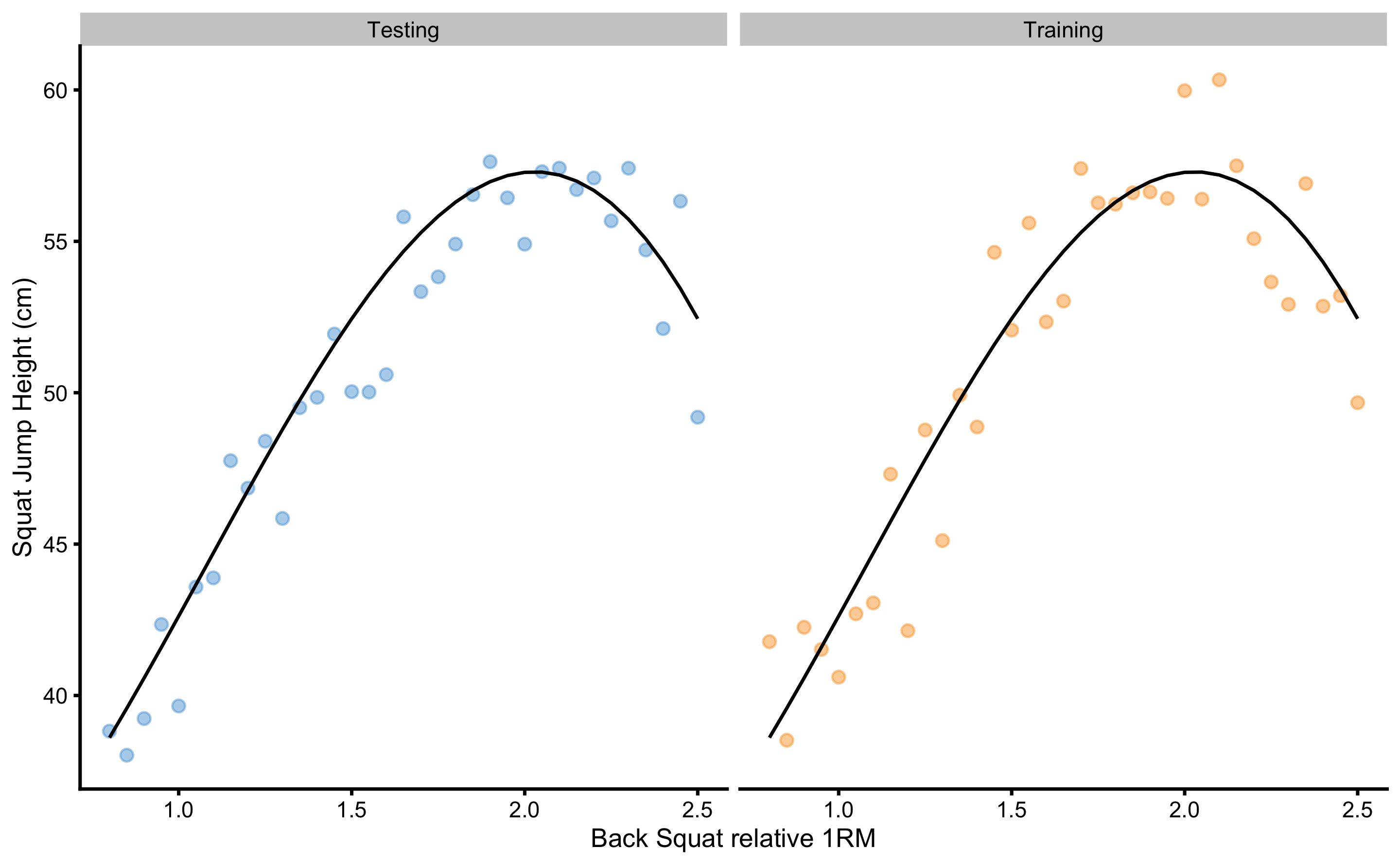
Figure 3.1: Two samples simulated from the known DGP. Black line represents systematic component of the DGP and it is equal for both training and testing samples. Observations vary in the two samples due stochastic component in the DGP

Model used to predict SJ from BS will be polynomial linear regression. Equation (3.3) explains first, second, and third degree polynomial linear regression function and provides a form for n-degree polynomials. Please, note that first degree polynomial function represents simple linear regression.

\[\begin{equation} \begin{split} \hat{y_i} &= \hat{\beta}_0 + \hat{\beta}_1 x_i^1 \\ \hat{y_i} &= \hat{\beta}_0 + \hat{\beta}_1 x_i^1 + \hat{\beta}_2 x_i^2 \\ \hat{y_i} &= \hat{\beta}_0 + \hat{\beta}_1 x_i^1 + \hat{\beta}_2 x_i^2 + \hat{\beta}_3 x_i^3 \\ \hat{y_i} &= \hat{\beta}_0 + \hat{\beta}_1 x_i^1 + \dots + \hat{\beta}_n x_i^n \end{split} \tag{3.3} \end{equation}\]

Increasing polynomial degrees increases the flexibility of the polynomial regression model, and thus can represent tuning parameter that we can select based on the model performance. In other words, we might be interested in finding polynomial degree that minimized model error (or maximize model fit). Figure 3.2 contains model performance on the training data for polynomial degrees ranging from 1 to 20.

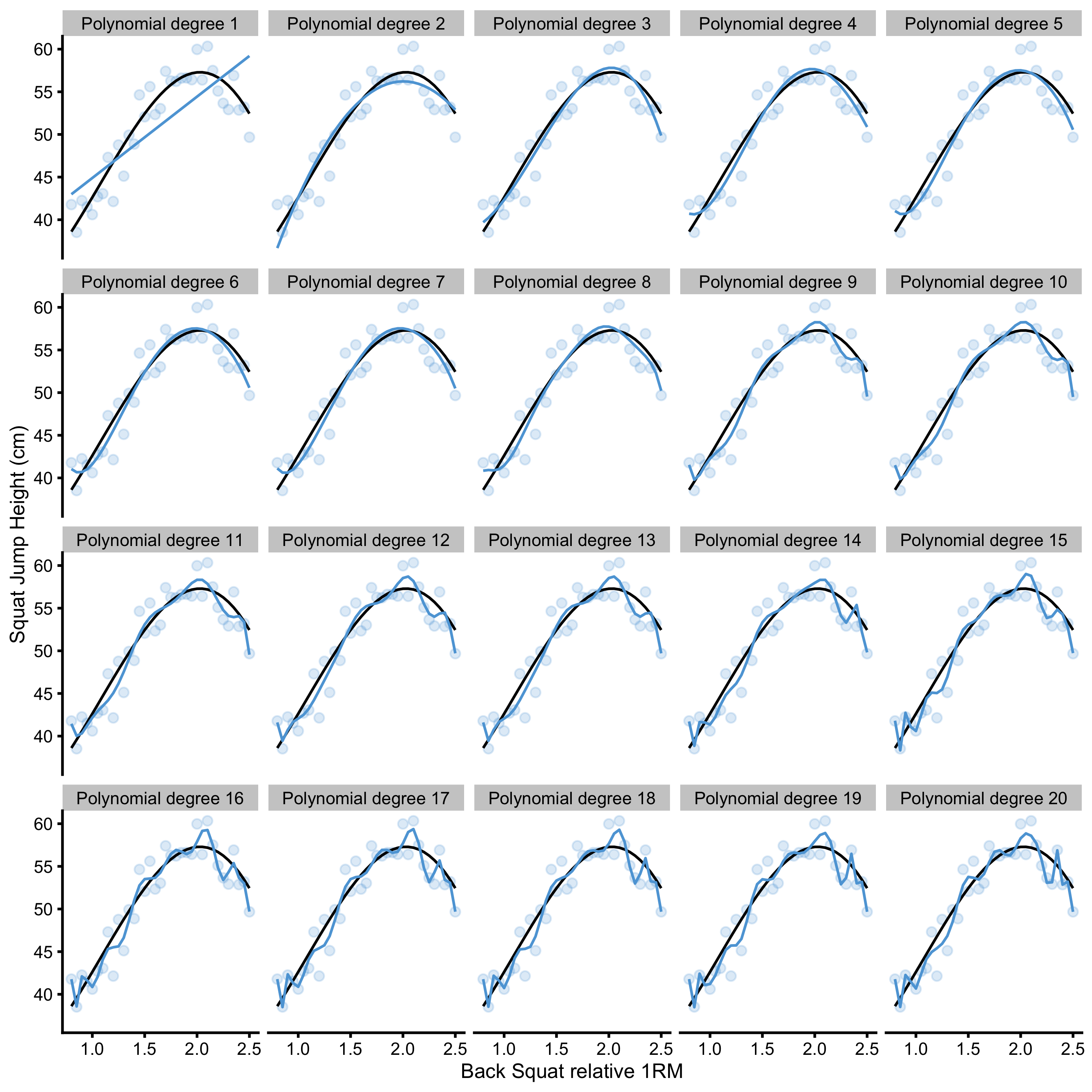
Figure 3.2: Model fit with varying polynomial degrees. More degrees equals better model fit

As can be seen from the Figure 3.2, the more flexible the model (or the higher the polynomial degree) the better it fits the data. But how do these models perform on the unseen, testing data sample? In order to quantify model performance, RMSE metric is used. Figure 3.3 demonstrates performance of the polynomial regression model on the training and testing data sample across different polynomial degrees.

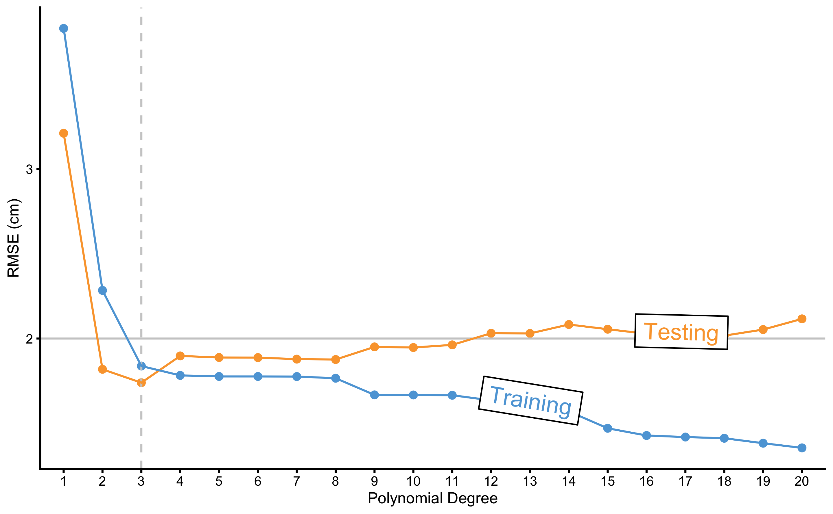
Figure 3.3: Testing and training errors across varying polynomial degrees. Model error is estimated with the RMSE metric, while polynomial degree represents tuning or flexibility parameter of the model. As can be noted from the figure, better training performance doesn’t imply better testing performance. Vertical dashed line represents the polynomial degree at which testing error is lowest. Polynomial degrees on the right of the vertical dashed line are said to overfit the data, while polynomial degree on the left are said to underfit the data

As can be seen from the Figure 3.3, models with higher polynomial degrees tend to overfit (indicated by performance better than the known irreducible error \(\epsilon\) visualized with the horizontal line at 2cm). Performance on the training data sample improves as the polynomial degrees increase, which is not the case with the performance on the testing data sample. There is clearly the best polynomial degree that has the best predictive performance on the unseen data. Polynomial degrees on the left of the vertical dashed line are said to underfit, while polynomial degrees on the right are said to overfit.

The take home message is that predictive performance on the training data can be too optimistic, and for evaluating predictive performance of the model, unseen data must be used, otherwise the model might overfit.

3.2 Cross-Validation

In order to evaluate predictive performance of the model, researchers usually remove some percent of data to be used as a testing or holdout sample. Unfortunately, this is not always possible (although it is recommended, particularly to evaluate final model performance, especially when there are multiple models and model tuning). One solution to these problems is cross-validation technique (92,111,206). There are numerous variations of the cross-validation, but the simplest one is n-fold cross validation (Figure 15). N-fold cross validation involve splitting the data into 5 to 10 equal folds and using one fold as a testing or hold-out sample while performing model training on the other folds. This is repeated over N-iteration (in this case 5 to 10) and the model performance is averaged to get cross-validated model performance.

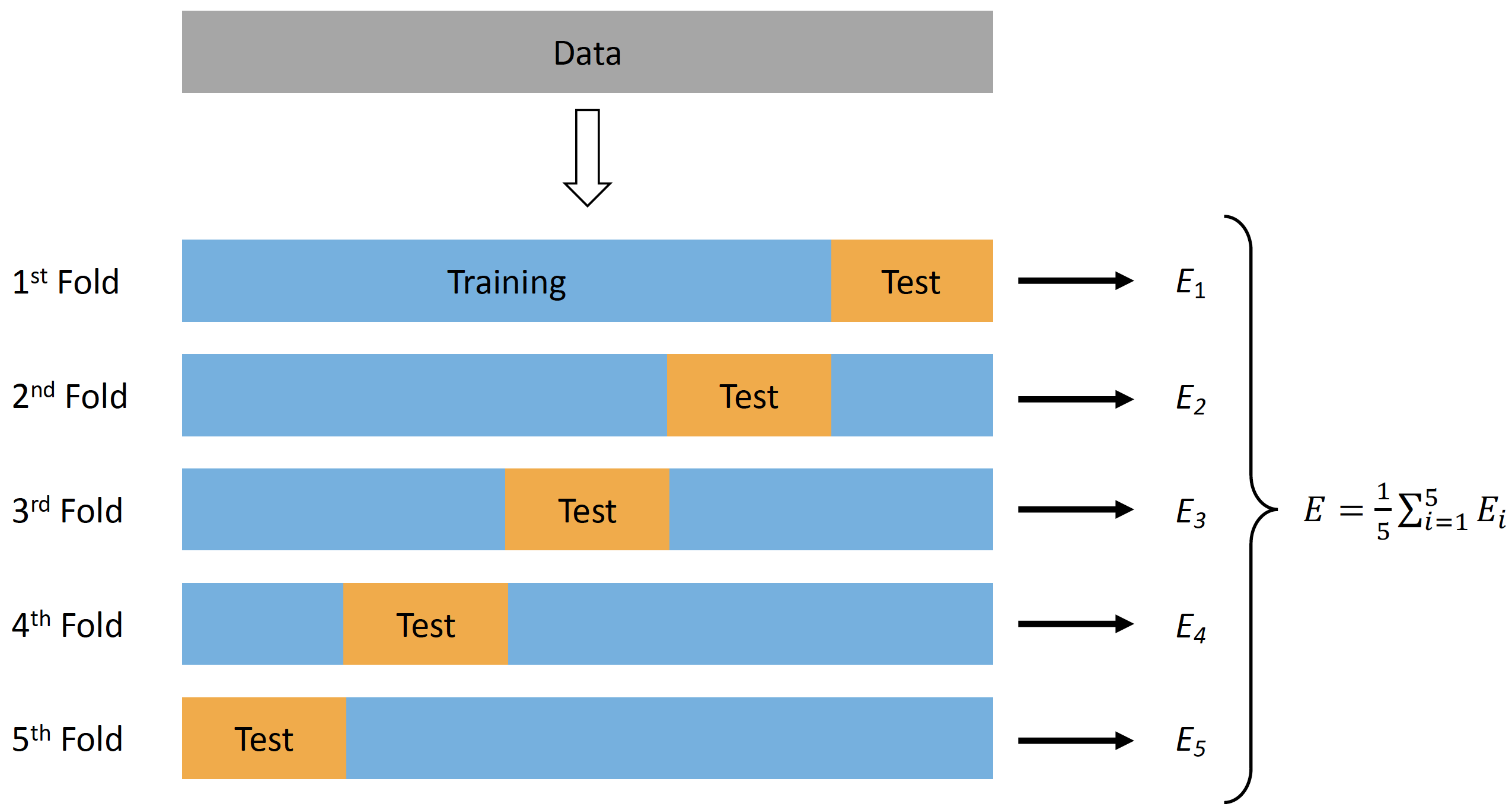
Figure 3.4: Cross-Validation

With predictive analysis and machine learning, different model’s tuning parameters are evaluated (as well as multiple different models) to estimate the one that gives the best predictive performance. It is thus important to utilize techniques such as cross-validation to avoid overfitting and too optimistic model selection.

Certain models, such as lasso, ridge regression, and elastic-net implement regularization parameters that penalizes the model complexity and are used as a tuning variable (92,111,206). This is useful in situations when there are a lot of predictors, and it is easy to overfit the model. Selecting the best regularization parameter that has the best cross-validated performance helps in simplifying the model and avoiding the overfit. These topics are beyond the scope of this book, and interested readers are directed to references provided.

3.2.1 Sample mean as the simplest predictive model

We have already discussed in Sample mean as the simplest statistical model section that sample mean can be considered simplest model that describes a particular sample with the lowest RMSE. But can it be used for prediction?

Here is an example to demonstrate both sample mean as a predictive model, as well as to demonstrate cross-validation technique. Let’s assume that we have collected N=10 observations: 15, 19, 28, 28, 30, 57, 71, 88, 95, 97. Sample mean is equal to 52.8. If we assume that the sample mean represents our prediction for the observations, we can easily calculate prediction error for each observation, which is simple difference (column Error in the Table 3.1).

Table 3.1: Sample mean as prediction with associated prediction errors

Observed	Predicted	Error	Absolute Error	Squared Error
15	52.8	37.8	37.8	1428.84
19	52.8	33.8	33.8	1142.44
28	52.8	24.8	24.8	615.04
28	52.8	24.8	24.8	615.04
30	52.8	22.8	22.8	519.84
57	52.8	-4.2	4.2	17.64
71	52.8	-18.2	18.2	331.24
88	52.8	-35.2	35.2	1239.04
95	52.8	-42.2	42.2	1780.84
97	52.8	-44.2	44.2	1953.64

Besides simple difference, Table 3.1 provides errors (or losses) using two common loss functions (see Sample mean as the simplest statistical model section in Description chapter): absolute loss (column Absolute Error) and quadratic loss (column Squared Error).

We need to aggregate these errors or losses into a single metric using the cost function. If we calculate the mean of the prediction errors (column Error in the Table 3.1), we are going to get 0. This is because the positive and negative errors cancel each other out for the sample mean estimator. This error estimator is often referred to as mean bias error (MBE) or simply bias and is often used in validity and reliability analysis (see Validity and Reliability sections).

If we take the mean of the absolute prediction errors (column Absolute error in the Table 3.1) we are going to get mean absolute error (MAE) estimator, which is in this example equal to 28.8.

If we take the mean of the squared prediction errors (column Squared error in the Table 3.1) we are going to get mean square error (MSE) estimator, often called variance in the case of describing sample dispersion. In this example MSE is equal to 964.36. To bring back MSE to the same scale with the observation scale, square root of the MSE is taken. This represents root mean square error (RMSE), which is equal to 31.05. As explained in Sample mean as the simplest statistical model section, sample mean represents statistical model of the central tendency with the lowest RMSE.

Aforementioned error estimators, MBE, MAE, MSE, and RMSE can be considered different cost functions. Which one should be used¹⁸? As always, it depends (33). Assuming Gaussian normal distribution of the errors, MSE and RMSE have very useful mathematical properties that can be utilized in modeling stochastic or random components (i.e. random error propagation and prediction error decomposition in Bias-Variance decomposition and trade-off section). This property will be utilized thorough this book and particularly in the Example of randomized control trial section when estimating random or stochastic component of the treatment effect. I personally prefer to report multiple estimators, including error estimators, which is also a strategy suggested by (33).

The are, of course, other loss and cost functions that could be used. For example, one might only use the maximal error (MaxErr) and minimal error (MinErr), rather than average. Discussion and review of these different metrics is beyond the scope of this book (for more information please check the package Metrics (64) and the following references (12,25,33,203)). Figure 3.5 visualize the most common loss functions that are used in both model training and as performance metrics. It is important to keep in mind that in the case of OLS regression, MSE (or RMSE) is minimized. It is thus important to make a distinction between cost function used in the optimization and model training (i.e. in OLS, parameters of the model are found so that MSE is minimized; in some machine-learning models Huber loss or Rigde loss¹⁹ is minimized; see Figure 3.5) versus cost function used as a performance metric (e.g. reporting pEquivalent, MaxErr or MinErr for OLS models).

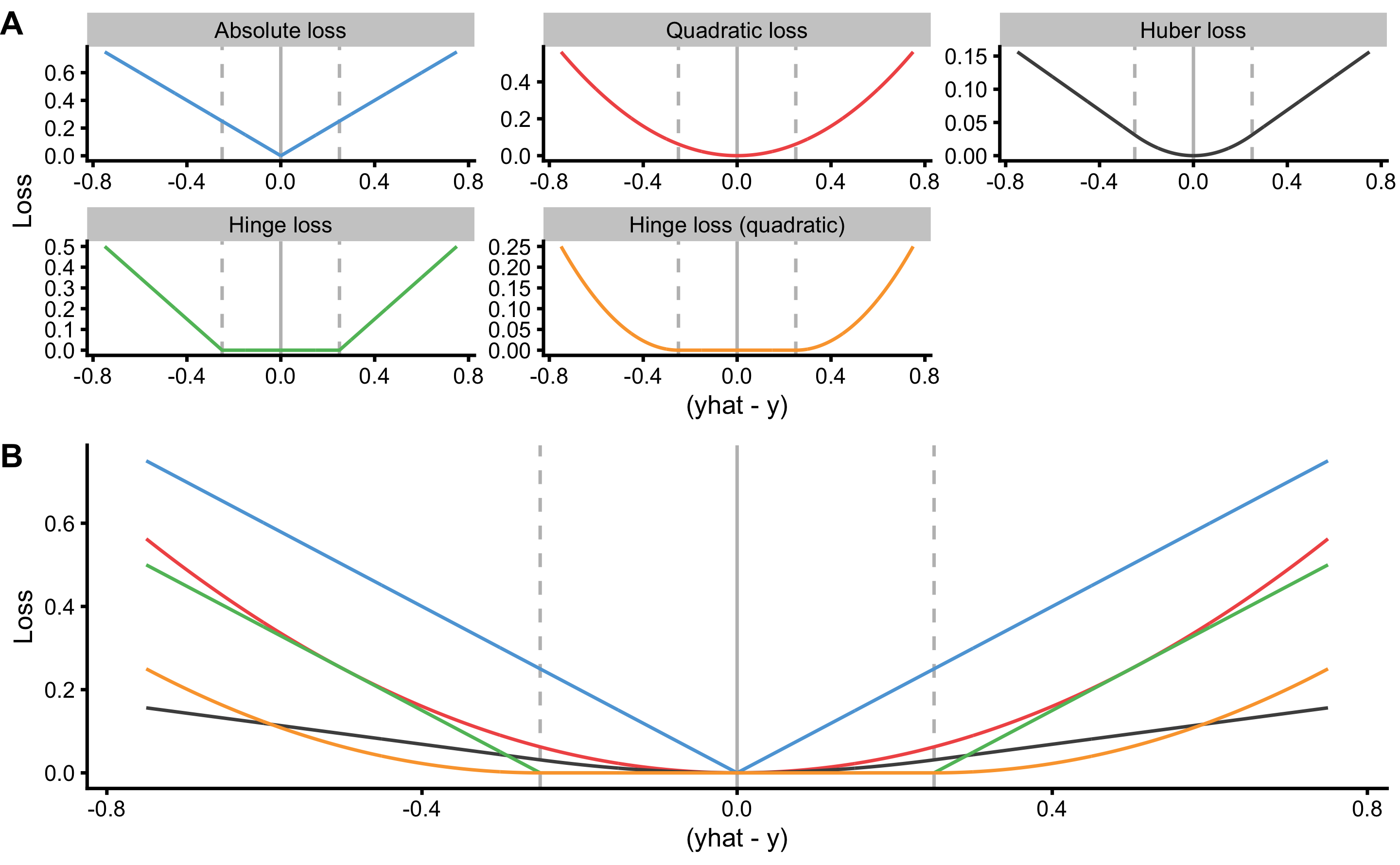
Figure 3.5: Common loss functions. A. Trellis plot of each loss function. B. Plot of all loss functions on a common scale. Huber loss is a combination of absolute and quadratic loss.

The take-away point is to understand that there are multiple performance metrics that can be utilized and it is best to report multiple of them.

Estimates for MBE, MAE, MSE²⁰, and RMSE represent training sample predictive performance since sample mean is estimated using this very sample. We are interested how sample mean, as predictive model, perform on the unseen data. Cross-validation is one method to estimate model performance on unseen data. Table 3.2 contains 3-fold cross-validation sample used to train the model (in this case estimate sample mean) and to evaluate the performance on unseen data.

Table 3.2: Example cross-validation using sample mean as the prediction model

Fold	Training sample	mean	Testing Sample	MBE	MAE	RMSE	MinErr	MaxErr
1	15 19 28 – 30 – 71 88 95 –	49.43	– – – 28 – 57 – – – 97	-11.24	25.52	30.44	-47.57	21.43
2	15 19 – 28 – 57 – 88 – 97	50.67	– – 28 – 30 – 71 – 95 –	-5.33	27.00	28.81	-44.33	22.67
3	– – 28 28 30 57 71 – 95 97	58.00	15 19 – – – – – 88 – –	17.33	37.33	37.73	-30.00	43.00

Since this is a small sample, we can repeat cross-validation few times. This is called repeated cross-validation. Let’s repeat 3-folds cross-validation for 5 repeats (Table 3.3).

Table 3.3: Example repeated cross-validation using sample mean as the prediction model

Repeat	Fold	Training sample	mean	Testing Sample	MBE	MAE	RMSE	MinErr	MaxErr
1	1	15 19 28 – 30 – 71 88 95 –	49.43	– – – 28 – 57 – – – 97	-11.24	25.52	30.44	-47.57	21.43
1	2	15 19 – 28 – 57 – 88 – 97	50.67	– – 28 – 30 – 71 – 95 –	-5.33	27.00	28.81	-44.33	22.67
1	3	– – 28 28 30 57 71 – 95 97	58.00	15 19 – – – – – 88 – –	17.33	37.33	37.73	-30.00	43.00
2	1	– 19 28 – 30 57 71 88 – –	48.83	15 – – 28 – – – – 95 97	-9.92	37.25	38.83	-48.17	33.83
2	2	15 – 28 28 – 57 – – 95 97	53.33	– 19 – – 30 – 71 88 – –	1.33	27.50	28.45	-34.67	34.33
2	3	15 19 – 28 30 – 71 88 95 97	55.38	– – 28 – – 57 – – – –	12.87	14.50	19.39	-1.63	27.37
3	1	– 19 28 28 30 57 71 88 – –	45.86	15 – – – – – – – 95 97	-23.14	43.71	44.66	-51.14	30.86
3	2	15 19 – – 30 – – 88 95 97	57.33	– – 28 28 – 57 71 – – –	11.33	18.17	21.84	-13.67	29.33
3	3	15 – 28 28 – 57 71 – 95 97	55.86	– 19 – – 30 – – 88 – –	10.19	31.62	31.94	-32.14	36.86
4	1	– 19 28 – 30 57 71 88 – 97	55.71	15 – – 28 – – – – 95 –	9.71	35.90	36.37	-39.29	40.71
4	2	15 – – 28 30 – 71 – 95 97	56.00	– 19 28 – – 57 – 88 – –	8.00	24.50	28.19	-32.00	37.00
4	3	15 19 28 28 – 57 – 88 95 –	47.14	– – – – 30 – 71 – – 97	-18.86	30.29	33.41	-49.86	17.14
5	1	15 19 – 28 – 57 – 88 95 97	57.00	– – 28 – 30 – 71 – – –	14.00	23.33	24.26	-14.00	29.00
5	2	15 – 28 28 30 – 71 88 95 –	50.71	– 19 – – – 57 – – – 97	-6.95	28.10	32.60	-46.29	31.71
5	3	– 19 28 – 30 57 71 – – 97	50.33	15 – – 28 – – – 88 95 –	-6.17	35.00	35.92	-44.67	35.33

To calculate cross-validated prediction performance metrics, average of testing MBE, MAE, RMSE, MinErr, and MaxErr is calculated and reported as cvMBE, cvMAE, cvRMSE, cvMinErr, and cvMaxErr (Table 3.4). Prediction performance metrics don’t need to be averaged across cross-validation samples and can be instead estimated by binding (or pooling) all cross-validated samples together (i.e. target variable and predicted target variable). More about this at the end of this chapter in Practical example: MAS and YoYoIR1 prediction section.

Table 3.4: Cross-validated prediction performance metrics (estimators)

cvMBE	cvMAE	cvRMSE	cvMinErr	cvMaxErr
0.21	29.32	31.52	-35.29	31.37

As can be seen from the Table 3.4, all performance metrics estimated using repeated cross-validation are larger than the when estimated using the training data (full sample). Utilizing cross-validated estimates of performance (or error) should be used over training estimates when discussing predictive performance of the models. Unfortunately, this is almost never the case in sport science literature, where prediction is never estimated on unseen data and the model performance estimates can suffer from over-fitting.

Using sample mean as predictive model represents simplistic example, although this type of model is usually referred to as baseline model. Baseline models are used as benchmarks or anchor when discussing performance of more elaborate and complex predictive models. We will come back to these at the end of this section when we will perform predictive analysis of the linear regression model used in Magnitude-based estimators section for predicting MAS from YoYoIR1 (and vice versa) tests.

3.3 Bias-Variance decomposition and trade-off

Prediction error can be decomposed into two components, reducible and irreducible error²¹. Reducible error is the error that can be reduced with a better model, while irreducible error is the unknown error inherent to the DGP itself (92). Reducible error can be further divided into \(Bias^2\) and \(Variance\) (Figure 3.6 and Equation (3.4)).

\[\begin{equation} \begin{split} Prediction \; error &= Reducible \; error + Irreducible \; error \\ Prediction \; error &= (Bias^2 + Variance) + Irreducible \; error \end{split} \tag{3.4} \end{equation}\]

\(Bias^2\) represents constant or systematic error, which is introduced by approximating a real-life problem, which may be extremely complicated, by a much simpler model (92). \(Variance\) represents variable or random error, and refers to the amount by which model parameters would change if we estimated it by using a different training data set (92).

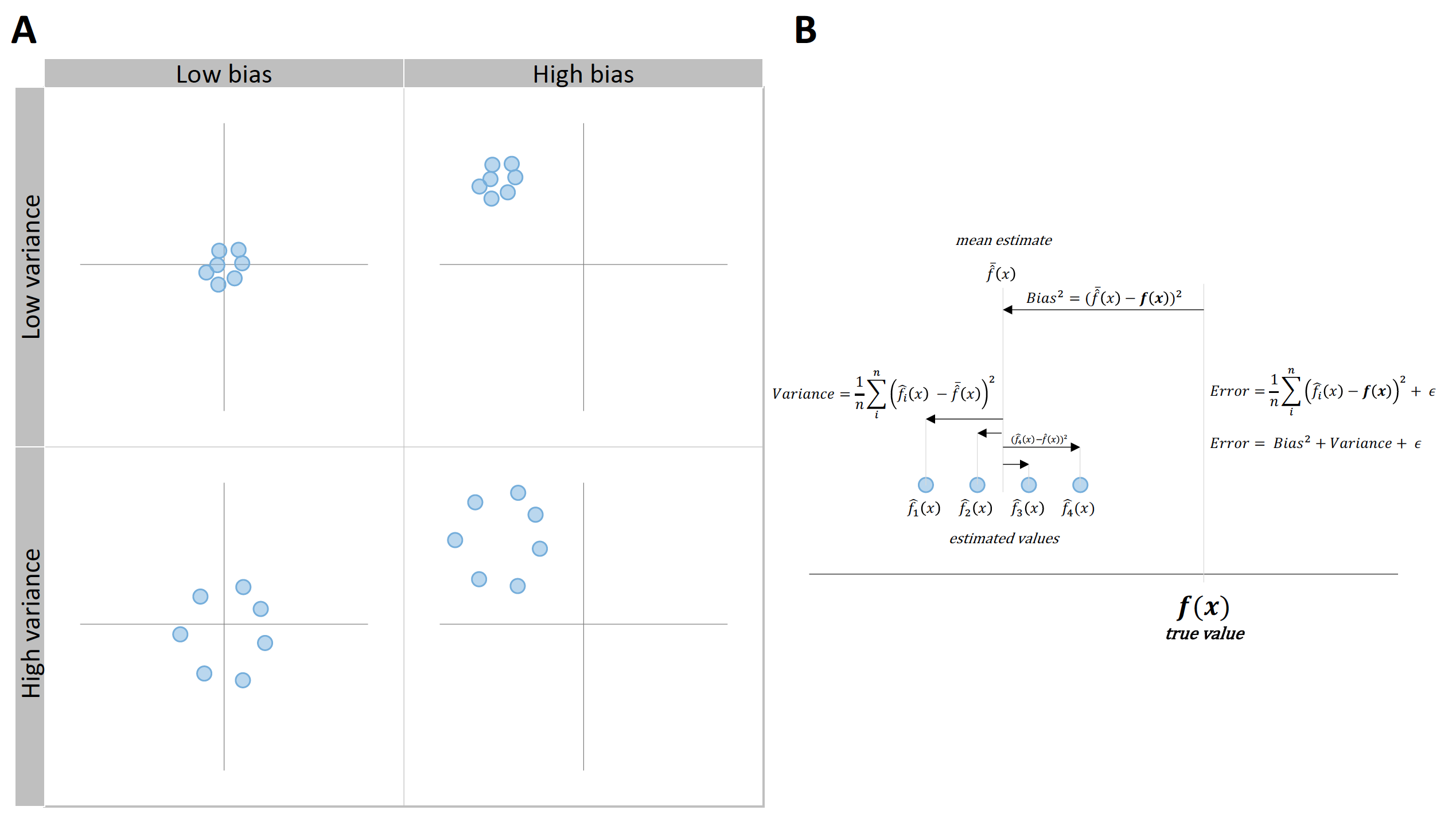
Figure 3.6: Bias and variance decomposition of the error. A. Visual representation of \(Bias^2\) and \(Variance\) using the shooting target. B. Error can be decomposed to \(Bias^2\), \(Variance\), and \(Irreducible \: error\), where \(Bias^2\) represents constant or systematic error and \(Variance\) represents variable or random error

To understand this concept, we need to run a simulation using known relationship between BS and SJ (see Figure 3.1, Figure 3.2, and Equation (3.2)). Prediction error decomposition to bias and variance is done for a single data point. To do that we need to differentiate between the following variables:

• \(x\) predictors. In our case we only have one \(x\) predictor - \(BS\) and we will use \(BS = 1.75\) for this simulation
• \(y_{true}\) value for a particular \(x\) values. In our case \(SJ\) variable represents target variable \(y\), which is equal to \(SJ = 30 + 15\times BS\times\sin(BS)\) or \(SJ=55.83\)cm. Both \(x\) and \(y_{true}\) values are constant across simulations
• \(y_{observed}\) represents observed \(y\) which differs from \(y_{true}\) due stochastic component \(\epsilon\). This implies that \(y_{observed}\) randomly varies across simulations. The equation for \(y_{observed}\) is: \(SJ = 30 + 15\times BS\times\sin(BS) + \mathcal{N}(0,\,2)\). Error \(\epsilon\) represents irreducible error, because it is inherent to DGP and it is equal to \(\mathcal{N}(0,\,2)\).
• \(y_{predicted}\) represents model prediction using the training sample of \(x\) and \(y_{observed}\) values.

For every simulation (N=200 simulations in total), the whole sample of N=35 observations is generated from the known DGP. This includes \(x\), \(y_{true}\), and \(y_{observed}\) variables. Polynomial regression models (from 1 to 20 polynomial degrees) are being fitted (or trained) using \(x\) predictors (in our case \(BS\) variable) and \(y_{observed}\) as our target variable. True \(y\) (\(y_{true}\)) is thus unknown to the model, but only to us. After models are trained, we estimate \(y_{predicted}\) using \(BS = 1.75\), for which the \(y_{true}\) is equal to \(SJ=55.83\)cm.

Table 3.5 contains results of the first 10 simulations for 2nd degree polynomial model.

Table 3.5: Results of first 10 simulations for 2nd degree polynomial linear regression model

sim	model	x	y_true	y_observed	y_predicted
1	2	1.75	55.83	54.65	55.27
2	2	1.75	55.83	53.80	55.34
3	2	1.75	55.83	56.03	55.34
4	2	1.75	55.83	55.71	55.68
5	2	1.75	55.83	55.52	54.91
6	2	1.75	55.83	57.55	55.81
7	2	1.75	55.83	52.03	55.08
8	2	1.75	55.83	56.35	55.92
9	2	1.75	55.83	54.05	54.64
10	2	1.75	55.83	58.16	55.57

To estimate reducible error, MSE estimator is used (Equation (3.5).

\[\begin{equation} Reducible \: error = \frac{1}{n_{sim}}\Sigma_{j=1}^{n_{sim}}(y_{predicted_{j,x=1.75}} - y_{true_{x=1.75}})^2 \tag{3.5} \end{equation}\]

Reducible error can be decomposed to \(Bias^2\) and \(Variance\), or systematic error and variable or random error. \(Bias^2\) is squared difference between \(y_{true}\) and mean of \(y_{predicted}\) across simulations (Equation (3.6)).

\[\begin{equation} Bias^2 = (\frac{1}{n_{sim}}\Sigma_{j=1}^{n_{sim}}(y_{predicted_{j, x=1.75}}) - y_{true_{x=1.75}})^2 \tag{3.6} \end{equation}\]

\(Variance\) represents, pretty much, SD of the of the \(y_{predicted}\) and it is an estimate of how much the predictions vary across simulations (Equation (3.7)).

\[\begin{equation} Variance = \frac{1}{n_{sim}}\Sigma_{j=1}^{n_{sim}}(\bar{y_{predicted_{x=1.75}}} - y_{predicted_{j, x=1.75}})^2 \tag{3.7} \end{equation}\]

Reducible error is thus equal to the sum of \(Bias^2\) and \(Variance\).

If you remember from Description section, \(Bias^2\) and \(Variance\) are nothing more than measure of central tendency (i.e. systematic or constant error) and measure of spread (i.e. variable or random error). Figure 3.6 also illustrates this concept.

Irreducible error is estimated using MSE as well (Equation MSE-irreducible-error).

\[\begin{equation} Irreducible \: error = \frac{1}{n_{sim}}\Sigma_{j=1}^{n_{sim}}(y_{observed_{x=1.75}} - y_{true_{x=1.75}})^2 \tag{3.8} \end{equation}\]

Since we know that the stochastic error in the DGP is normally distributed with SD=2cm, expected irreducible error should be around 4cm (this is because MSE is mean squared error, and RMSE, which is equivalent to SD, is calculated by doing square root of MSE). This might not be exactly 4cm due sampling error which is the topic of Statistical inference section.

As explained in Equation (3.4), \(Prediction \: error\) is equal to sum of \(Bias^2\), \(Variance\) and \(Irreducible \: error\). Table contains estimated aforementioned errors using all 200 simulations for 2nd degree polynomial linear regression.

Table 3.6: Calculated errors for all 200 simulations for 2nd degree polynomial linear regression

model	x	y_true	Prediction error	Bias^2	Variance	Irreducible error
2	1.75	55.83	5.17	0.09	0.21	4.87

This decomposition of errors is one useful mathematical property when using squared erors that I alluded to in the Cross-Validation section when discussing prediction error metrics.

If we perfrom this analysis for each degree of polynomial fit, we will estimate prediction error, as well as \(Bias^2\) and \(Variance\) across model complexity (i.e. polynomial degrees). This is visualized in the Figure 3.7.

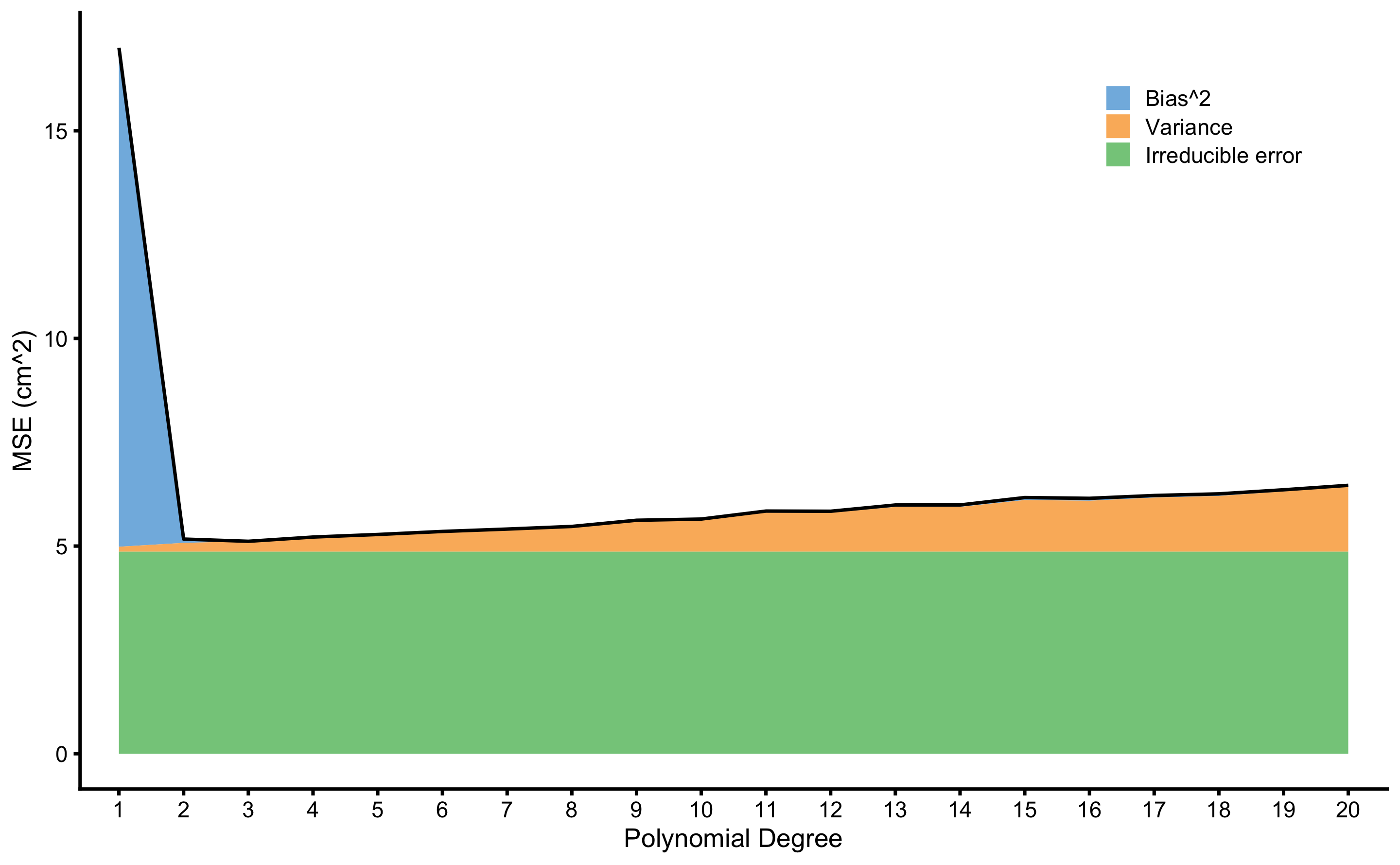
Figure 3.7: Bias and Variance error decomposition. \(Prediction \: error\) is indicated with the black line, and is decomposed to \(Bias^2\), \(Variance\), and \(Irreducible \: error\). These are represents with areas of different color

Beside decomposition of \(Prediction \: error\) to \(Bias^2\), \(Variance\) and \(Irreducible \: error\), it is important to notice the trade-off between \(Bias^2\) and \(Variance\). Linear regression models with lower polynomial degree, particularly 1st degree which is simple linear regression, has higher \(Bias^2\) due imposed linearity of the model (we can say that linear regression model is more biased). As \(Bias^2\) decreases with more flexible models (i.e. higher polynomial degree), \(Variance\) increase due model being too jumpy across simulations. To achieve best prediction (or the lower \(Prediction \: error\)) a balance between \(Bias^2\) and \(Variance\) needs to be found, both within a particular model and across models. The free lunch theorem (111,206) states that there is no single model that is the best across all different sets of problems. One needs to evaluate multiple models²² to estimate which one is the best for a particular problem at hand.

To estimate \(Bias^2\) and \(Variance\), true DGP must be known. Unfortunately, we do not know these for the real world problems, only for simulations. But even when we do not know \(y_{true}\) values (and thus \(Irreducible \: error\)), concepts of \(Bias^2\) and \(Variance\) can be applied in cross-validation samples (particularly when using multiple repeats) and can estimated using \(y_{observed}\). I will provide one such analysis in Practical example: MAS and YoYoIR1 prediction section.

3.4 Interpretability

As explained, predictive models put predictive performance over explanation of the underlying DGP mechanism (which is treated as a black box). However, sometimes we might be interested in which predictor is the most important, how do predictions change when particular predictor changes, or why²³ model made a particular prediction for a case of interest (111,137,157). Model interpretability can be defined as the degree to which a human can understand the cause of a decision (15,132,137). Some models are more inherently interpretable (e.g. linear regression) and some are indeed very complex and hard to interpret (e.g. random forest or neural networks). For this reason, there are model-agnostic techniques that can help increase model interpretability.

Excellent book and R (154) package by Christoph Molnar (137,138) demonstrates a few model-agnostic interpretation techniques. One such technique is estimating which predictor is the most important (variable importance). One method for estimating variable importance involves perturbing one predictor and estimating the change in model performance. The predictor whose perturbing causes the biggest change in model performance can be considered the most important (111,137). There are others approaches for estimating variable importance (63). Those interested in further details can also check vip (61) R (154) package.

One might be interested in how the predicted outcome changes when particular predictor changes. Techniques such as partial dependence plot (PDP), individual conditional expectation (ICE) and accumulated local effects (ALE) can be helpful in interpreting the effect of particular predictor on predicted outcome (60,62,137,138,207). Similar techniques are utilized in Prediction as a complement to causal inference section. Interested readers are also directed toward visreg (26) and effects (49–51) R (154) packages for more information about visualizing models.

It is important to keep in mind that these model-agnostic explanations should not be automatically treated as causal explanations (148,150), but as mere association and descriptive analysis that can still be useful in understanding and interpreting the underlying predictive black-box. They are not without problems, such as correlated variables, interactions and other issues (7).

According to Judea Pearl (148,150), prediction models should belong to the first level of ladder of causation²⁴, which represents simple “curve fitting”. Although in under special conditions these techniques can have causal interpretation (207).

The distinctions, similarities and issues between predictive modeling, machine learning and causal inference is currently hot topic in debates between machine learning specialists, statisticians and philosophers of science and it is beyond the scope of this book to delve into the debate. Interested readers are directed towards work by Miguel Hernan (73–77), Judea Pearl (147–150), Samantha Kleinberg (104,105) and others (27,103,163,177,187,206). The next Causal Inference section introduces the causal inference as a specific task of statistical modeling.

3.5 Magnitude-based prediction estimators

Similar to the magnitude-based estimators from Describing relationship between two variables section, one can utilize target variable SESOI to get magnitude-based estimates of predictive performance of the model. Rather than utilizing RSE as an estimate of the model fit in the training data, one can utilize cross-validated RMSE (cvRMSE), SESOI to cvRMSE, as well as cross-validated proportion of practically equivalent residuals (cvPPER) estimators.

Continuing with the squat jump height and relative squat 1RM example, one can assume that the SESOI in the squat jump is ±1cm. For the sake of example, we can feature engineer (110,111) relative squat 1RM variable to include all 20 degree polynomials. This way, we have created 20 predictor variables. To avoid overfitting, elastic-net model (53) implemented in the caret R package (111,112) is utilized, as well as repeated cross-validation involving 3 splits repeated 10 times. Predictive model performance is evaluated by using cvRMSE, together with magnitude-based performance estimators (SESOI to cvRMSE and cvPPER).

Elastic-net model represents regression method that linearly combines the L1 and L2 penalties of the lasso and ridge methods, or alpha and lambda tuning parameters (53,92,111). Total of nine combinations of tuning parameters is evaluated using aforementioned repeated cross-validation, and the model with minimal cvRMSE is selected as the best one. Performance metrics of the best model are further reported. Table 3.7 contains cross-validated best model performance metrics together with model performance on the training data set.

Table 3.7: Common predictive metrics and magnitude-based predictive metrics. Metrics starting with cv indicate cross-validated performance metrics. Metrics without cv indicate performance metrics on the training data set, which is often more optimistic

SESOI (cm)	cvRMSE (cm)	SESOI to cvRMSE	cvPPER	RMSE (cm)	SESOI to RMSE	PPER
±1	2.19	0.91	0.33	1.99	1.01	0.38

Utilizing apriori known SESOI gives us practical anchor to evaluate predictive model performance. Reported SESOI to cvRMSE (0.91) as well as cvPPER (0.33) indicate very poor predictive performance of the model. In practical terms, utilizing relative squat 1RM doesn’t produce practically meaningful predictions given SESOI of ±1cm and the model as well as the data sample utilized.

Model performance can be visualized using the training data set (Figure 3.8). PPER estimator, for both cross-validate estimate and training data performance estimate, utilized SD of the residuals and provided SESOI. Grey band on panels A and B on Figure 3.8 represents SESOI, and as can be visually inspected, model residuals are much wider than the SESOI, indicating poor practical predictive performance.

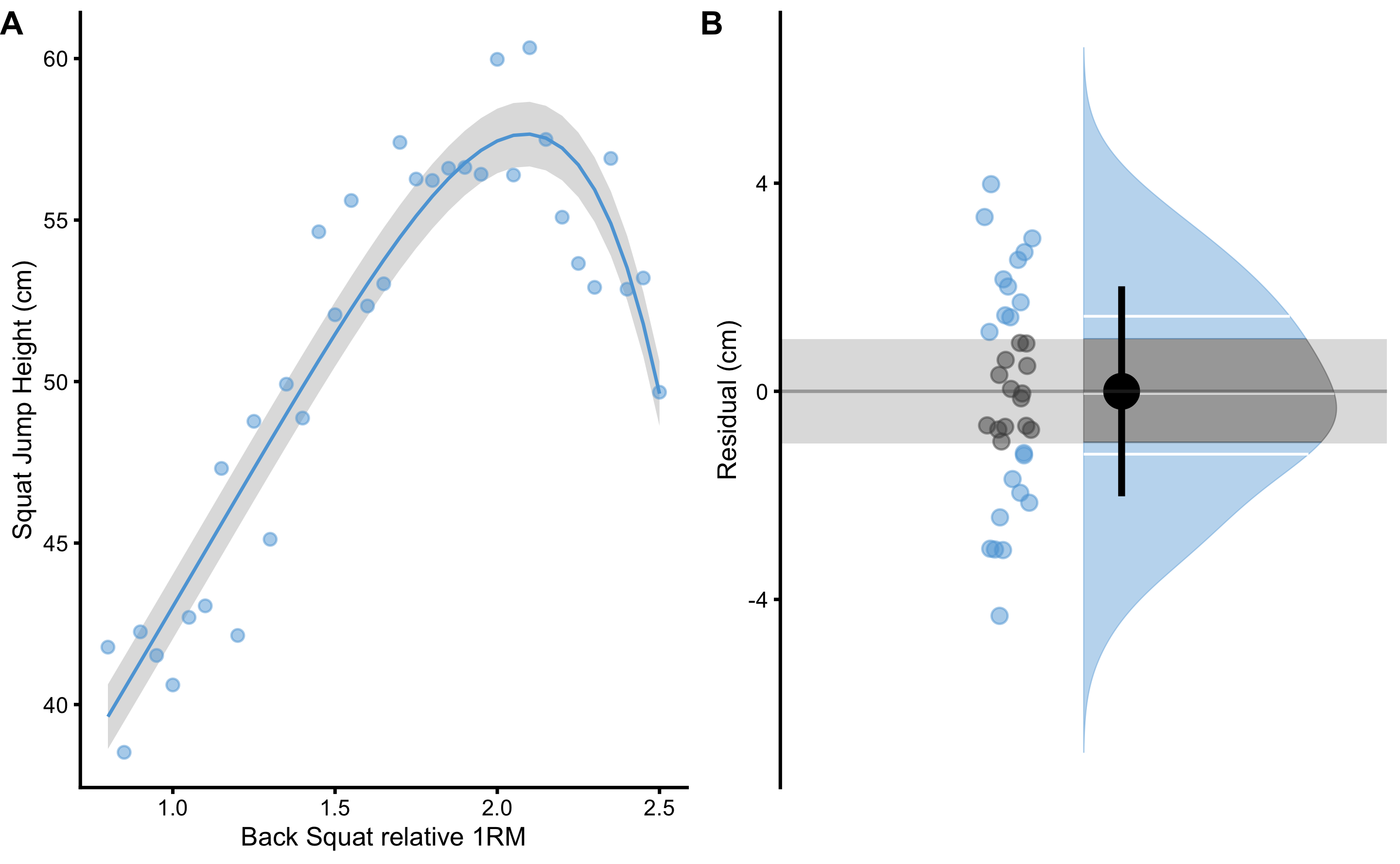
Figure 3.8: Model performance on the training data set. A. Model with the lowest cvRMSE is selected. SESOI is depicted as grey band around the model prediction (blue line). B. Residuals scatter plot. Residuals outside of the SESOI band (grey band) indicate prediction which error is practically significant. PPER represents proportion of residuals inside the SESOI band

Predictive tasks are focusing on providing the best predictions on the novel or unseen data without much concern about the underlying DGP. Predictive model performance can be evaluated by using magnitude-based approach to give insights into practical significance of the predictions. These magnitude-based prediction estimators, can be used to complement explanatory or causal inference tasks, rather than relying solely on the group-based and average-based estimators. This topic is further discussed in the Prediction as a complement to causal inference section.

3.6 Practical example: MAS and YoYoIR1 prediction

In Describing relationship between two variables we have used two physical performance tests, MAS and YoYoIR1, to showcase relationship or association between two variables. Besides mere association, we have stepped into the domain of prediction by utilizing magnitude-based estimators such as PPER and SESOI to RMSE. As you have learned so far in this section, these predictions were made on the training data set. Let’s implement concepts learned so far to estimate predictive performance on the unseen data. Why is this important? Although very simple model, we are interested in predicting MAS from YoYoIR1 test score for a new or unseen individual. For this reason, it is important to get estimates of model performance on the unseen athletes.

3.6.1 Predicting MAS from YoYoIR1

Let’s first estimate predictive performance when predicting MAS scores from the YoYoIR1 score using MAS SESOI ±0.5km/h and linear regression.

Figure 3.9 consists of two panels. Panel A depicts scatter plot between YoYoIR1 and MAS scores (black line represents linear model fit). Panel B depicts \(y_{predicted}\) (predicted or fitted MAS using simple linear regression; i.e. the black line on the panel A) against the model residuals \(y_{residual} = y_{predicted} - y_{observed}\), or Predicted MAS - MAS. The data points represent model performance on the full training data set.

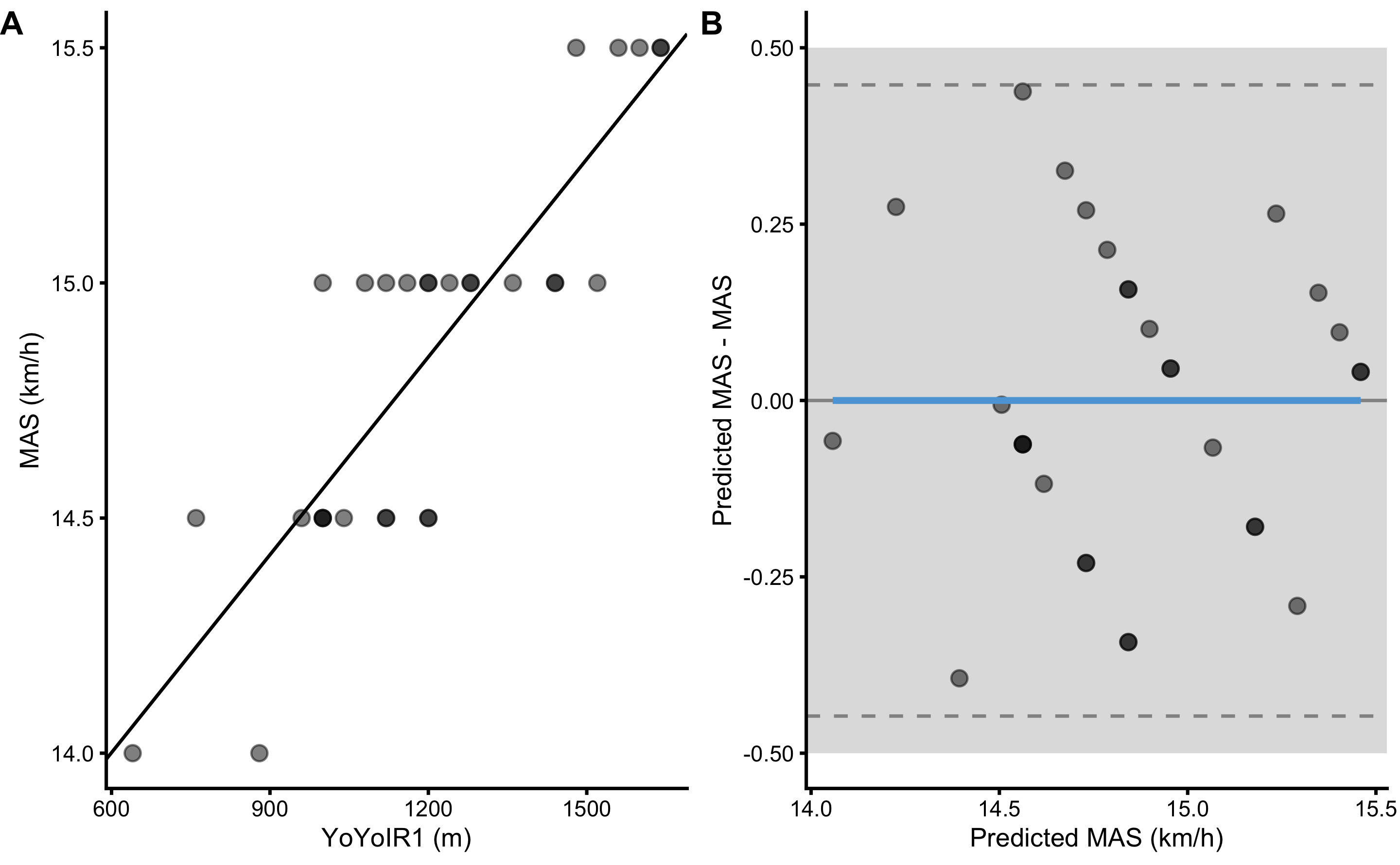
Figure 3.9: Scatter plot for simple linear regression between MAS and YoYoIR1 using the full training data sample. A. Scatter plot between MAS and YoYoIR1 scores. Black line indicates model prediction. B. Scatter plot between \(y_{predicted}\) (fitted or predicted MAS) against model residual \(y_{residual} = y_{predicted} - y_{observed}\), or Predicted MAS - MAS. Dotted lines indicate Levels of Agreement (LOA; i.e. upper and lower threshold that contain 95% of residuals distribution) and grey band indicates SESOI. Blue line indicate linear regression fit of the residuals and is used to indicate issues with the model (residuals)

Predictive performance for the full training data set is enlisted in the Table 3.8.

Table 3.8: Predictive performance using the full training data set

MBE	MAE	RMSE	PPER	SESOI.to.RMSE	R.squared	MinErr	MaxErr	MaxAbsErr
0	0.17	0.21	0.97	4.73	0.74	-0.44	0.39	0.44

But as already explained, these are not predictive performance estimators for the unseen data. To estimate how the model performs on the unseen data (i.e. unseen athletes in this case), cross-validation is performed using 3 folds and 5 repeats. Estimated predictive performance for every cross-validation sample is enlisted in the Table 3.9.

Table 3.9: Predictive performance for every repeated cross-validated sample

	fold	MBE	MAE	RMSE	PPER	SESOI to RMSE	R-squared	MinErr	MaxErr	MaxAbsErr
1	Fold1.Rep1	-0.13	0.27	0.29	0.87	3.42	0.62	-0.46	0.38	0.46
2	Fold1.Rep2	-0.04	0.13	0.14	0.99	7.15	0.87	-0.22	0.15	0.22
3	Fold1.Rep3	0.13	0.24	0.27	0.90	3.74	0.79	-0.27	0.49	0.49
4	Fold1.Rep4	-0.17	0.25	0.28	0.89	3.52	0.41	-0.51	0.26	0.51
5	Fold1.Rep5	0.08	0.20	0.24	0.92	4.20	0.77	-0.28	0.46	0.46
6	Fold2.Rep1	0.09	0.15	0.19	0.97	5.18	0.87	-0.27	0.37	0.37
7	Fold2.Rep2	0.05	0.20	0.24	0.93	4.16	0.71	-0.31	0.41	0.41
8	Fold2.Rep3	-0.14	0.18	0.22	0.96	4.65	0.81	-0.38	0.18	0.38
9	Fold2.Rep4	-0.02	0.13	0.17	0.98	5.92	0.75	-0.30	0.33	0.33
10	Fold2.Rep5	-0.07	0.21	0.27	0.89	3.76	0.27	-0.50	0.33	0.50
11	Fold3.Rep1	0.04	0.13	0.16	0.99	6.27	0.60	-0.20	0.31	0.31
12	Fold3.Rep2	-0.01	0.20	0.24	0.92	4.21	0.54	-0.45	0.34	0.45
13	Fold3.Rep3	0.02	0.15	0.21	0.95	4.74	0.51	-0.44	0.35	0.44
14	Fold3.Rep4	0.21	0.23	0.28	0.91	3.57	0.83	-0.06	0.53	0.53
15	Fold3.Rep5	-0.01	0.17	0.19	0.97	5.29	0.82	-0.32	0.34	0.34

As explained in Cross-Validation section, to calculate overall cross-validated performance, the mean is calculated for the performance metrics in the Table 3.9. Besides reporting the mean as the summary for predictive performances across cross-validated samples, SD, min, and max can be reported too. Another method of summarizing predictive performance over cross-validated samples would be to bind or pool all \(y_{observed}\) and \(y_{predicted}\) scores from the test samples together and then calculate overall predictive performance metrics. These pooled cross_validated \(y_{observed}\) and \(y_{predicted}\) can also be visualized using the residuals plot (Panel C in Figure 3.10).

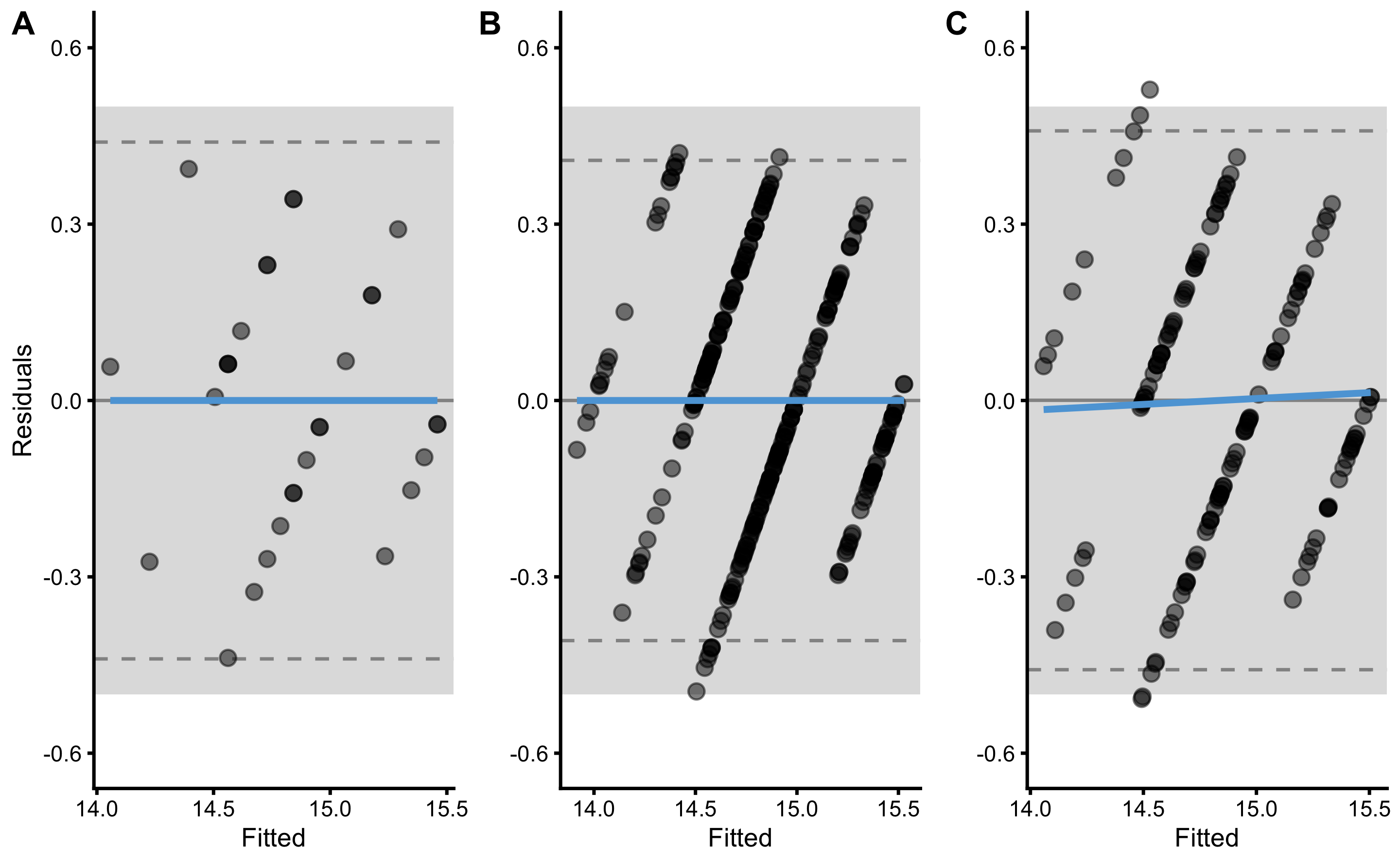
Figure 3.10: Residuals plot. A. Model residuals using the training data. This is exactly the same as panel B in Figure 3.9. B. Model residuals using the cross-validated training data. C. Model residuals using the cross-validated testing data.

As can be seen from the panels B and C in Figure 3.10, since we have used 5 repeats of the 3-fold cross-validations, each \(y_{observed}\) will have 5 assigned \(y_{predicted}\) scores. These can be used to estimate \(Bias^2\) and \(Variance\) as explained in the Bias-Variance decomposition and trade-off section. Since we do not know the \(y_{true}\) scores, we can only estimate \(Bias^2\) and \(Variance\) of the model for each \(y_{observed}\) using cross-validated \(y_{predicted}\). This is, of course, only possible if multiple repeats of cross-validation are performed. It bears repeating that this \(Bias^2\) and \(Variance\) decomposition of the prediction error using cross-validated \(y_{predicted}\) and \(y_{observed}\) are NOT the same as when using simulation and known DGP as done in Bias-Variance decomposition and trade-off section.

But these can be useful diagnostic tools for checking where the model fails (e.g. what particular observation might be problematic or outlier, as well how does \(Bias^2\) and \(Variance\) changes across \(y_{observed}\) continuum). These two concepts are depicted on Figure 3.11 and Figure 3.12.

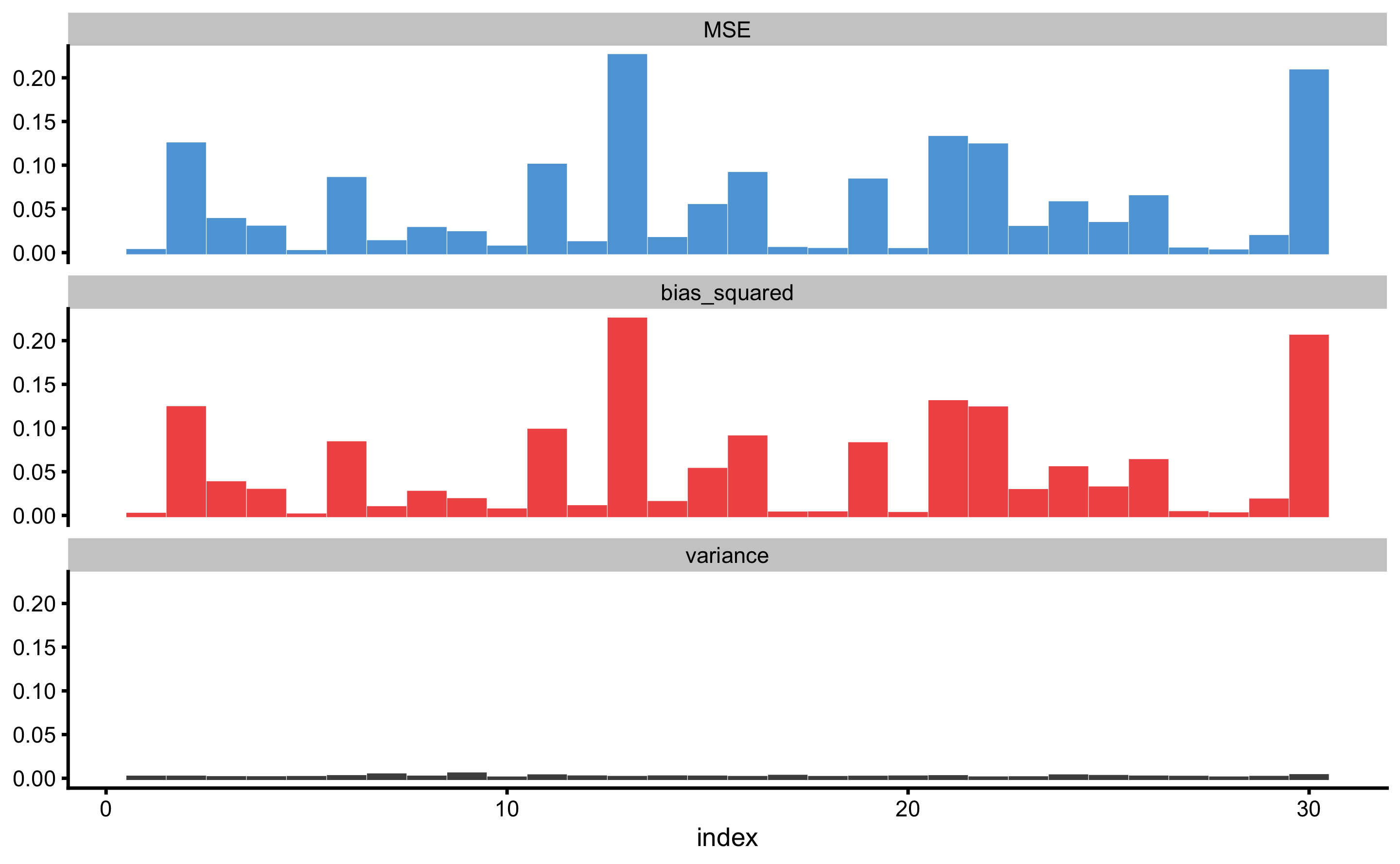
Figure 3.11: Prediction error (\(MSE\)), \(Bias^2\), and \(Variance\) across repeated cross-validated testing data. X-axis on the panels represents observation index, as in \(y_{i, observed}\)

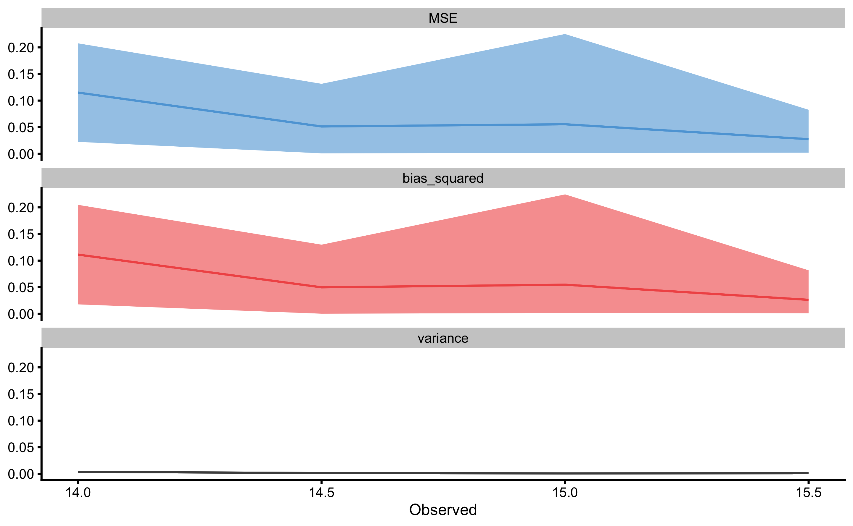
Figure 3.12: Prediction error (\(MSE\)), \(Bias^2\) and \(Variance\) across repeated cross-validated testing data. X-axis on the panels represent \(y_{observed}\). Since there might be multiple equal \(y_{observed}\), min and max are used and represent ribbon over mean (indicated by line)

Since \(Bias\) and \(Variance\) represent a quantitative summary of the residuals across cross-validations, the residuals and predicted observations across cross-validation testing folds can be visualized in more details as depicted on Figures 3.13 and 3.14.

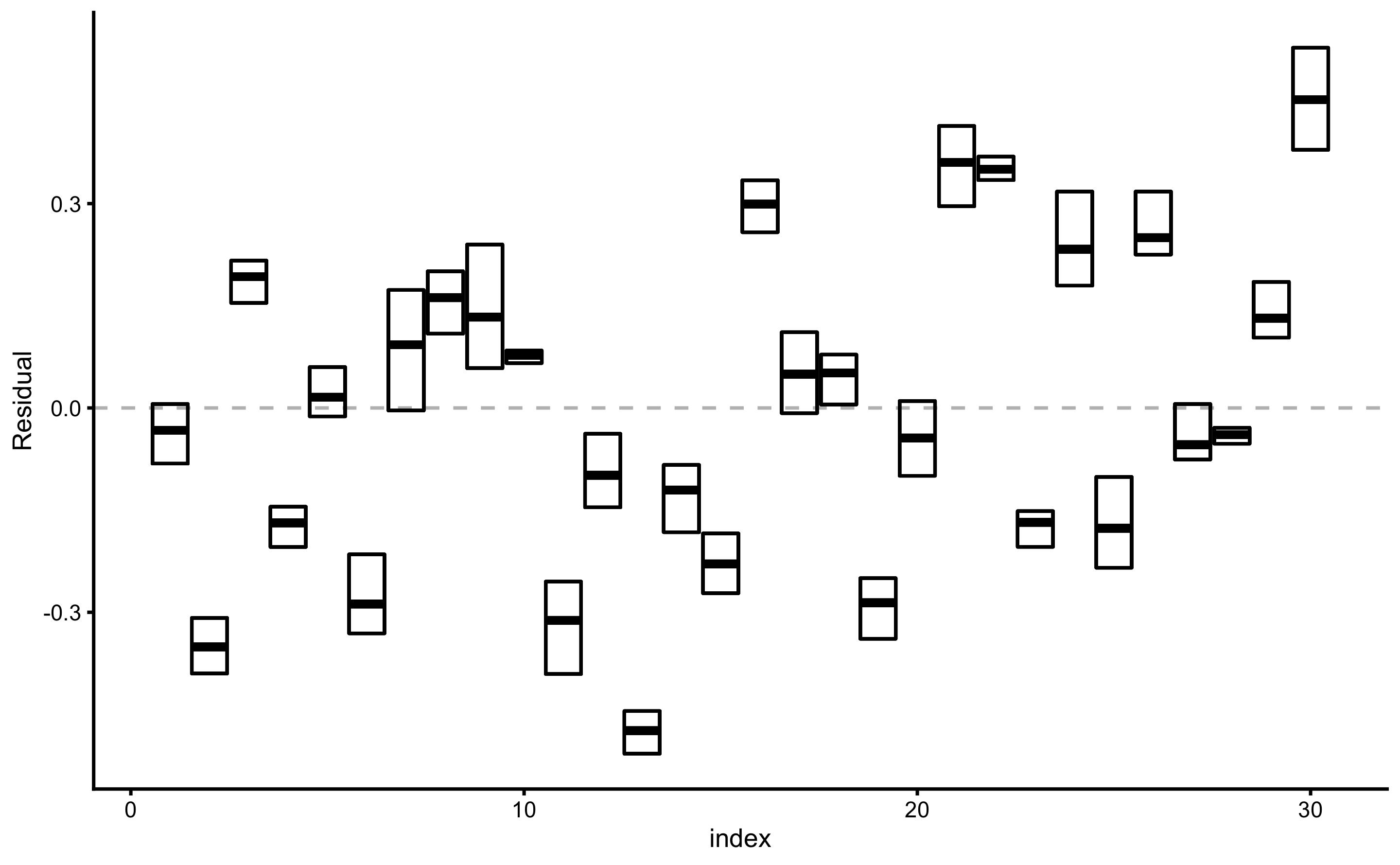
Figure 3.13: Testing prediction residuals across cross-validation folds summarized with cross-bars for every observation. Cross-bars represent ranges of testing residuals for each observation, while horizontal bar represent mean residual. The length of the bar represents \(Variance\), while distance between horizontal dashed line and horizontal line in the cross-bar (i.e. mean residual) represents \(Bias\).

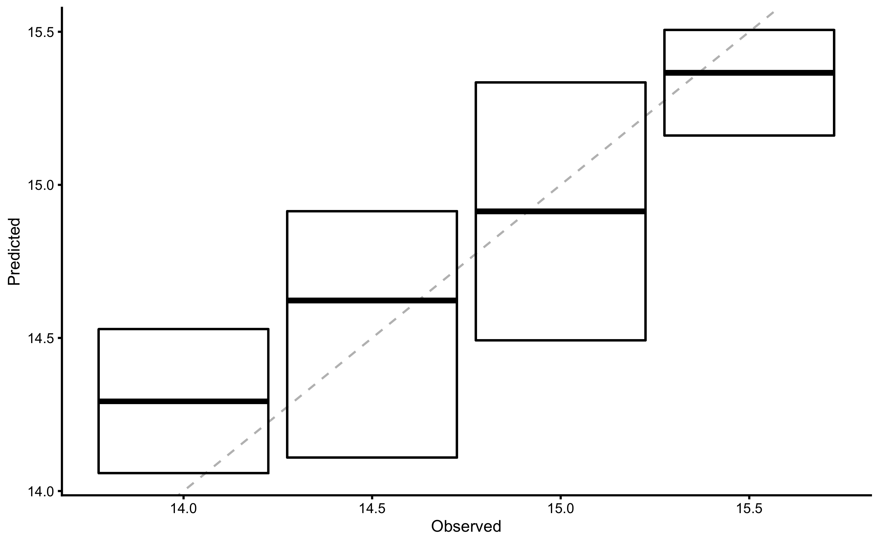
Figure 3.14: Testing prediction residuals across cross-validation folds summarized with cross-bars for every observation value. Cross-bars represent ranges of testing residuals for each observation, while horizontal bar represent mean residual. The length of the bar represents \(Variance\), while distance between horizontal dashed line and horizontal line in the cross-bar (i.e. mean residual) represents \(Bias\).

Cross-validated, pooled, and full training data set predictive performance metrics can be found in the Table 3.10. Please note that the pooled predictive performance metrics are in the column testing.pooled.

Table 3.10: Predictive performance summary

metric	training	training.pooled	testing.pooled	mean	SD	min	max
MBE	0.00	0.00	0.00	0.00	0.10	-0.17	0.21
MAE	0.17	0.17	0.19	0.19	0.05	0.13	0.27
RMSE	0.21	0.21	0.23	0.23	0.05	0.14	0.29
PPER	0.97	0.98	0.97	0.94	0.04	0.87	0.99
SESOI to RMSE	4.73	4.83	4.33	4.65	1.12	3.42	7.15
R-squared	0.74	0.75	0.68	0.68	0.18	0.27	0.87
MinErr	-0.44	-0.49	-0.51	-0.33	0.13	-0.51	-0.06
MaxErr	0.39	0.42	0.53	0.35	0.10	0.15	0.53
MaxAbsErr	0.44	0.49	0.53	0.41	0.09	0.22	0.53

Summary from the Table 3.10 as well as the individual cross-validated sample predictive performance from the Table 3.9 are visually represented in the Figure 3.15).

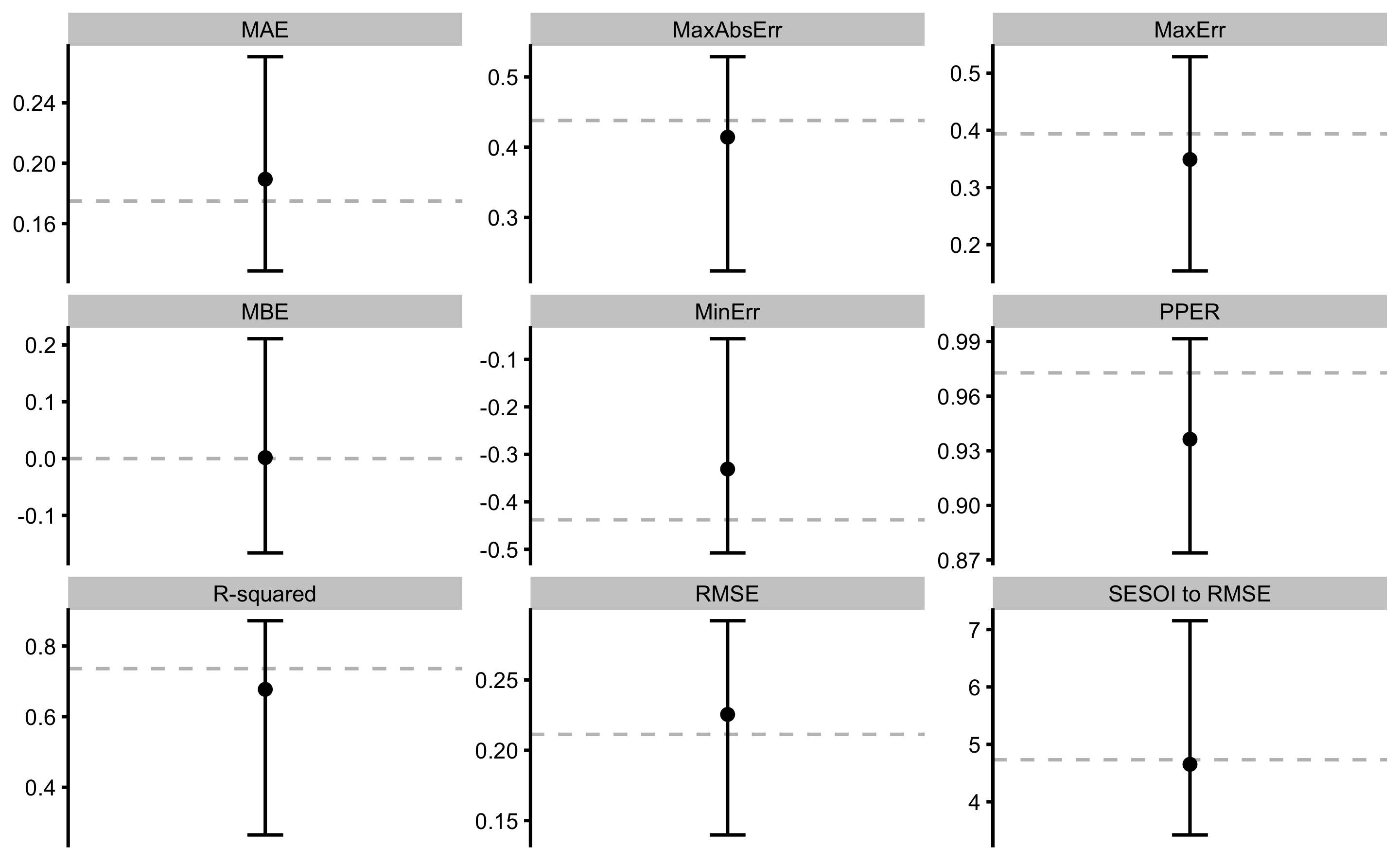
Figure 3.15: Cross-validated model performance. Dot and line bar indicate mean, min and max of the cross-validated performance. Dotted line indicate model performance on the training data set.

As can be seen from the Figure 3.15, cross-validated prediction performance metrics do not differ much²⁵ from the metrics estimated using the full training sample (calculated in Describing relationship between two variables section and in the Table 3.8, and indicated by the dotted horizontal line in the Figure 3.15). For some more complex models, these differences can be much larger and are clear indication of the model over-fitting.

Overall, predicting MAS from the YoYoIR1 score, given the data collected, SESOI of ±0.5km/h, and linear regression as a model, is practically excellent. Please note that prediction can be practically useful (given SESOI) (PPER; CV from 0.87 to 0.99) even when R-squared is relatively low (CV from 0.27 to 0.87). And the vice versa in some cases. That’s the reason why we need to utilize magnitude-based estimators as a complement of contemporary estimators such as R-squared, RSE, and RMSE.

3.6.2 Predicting YoYoIR1 from MAS

As shown in Describing relationship between two variables, predicting YoYoIR1 from MAS scores was not practically useful (or precise enough). But for the sake of completeness, let’s perform cross-validated prediction (using 3 folds and 5 repeats). YoYoIR1 SESOI is taken to be ±40m.

Figure 3.16 depicts modified Bland-Altman plot for predictions using the full training data set. Visual inspection demonstrates that many points are outside of SESOI band, indicating poor practically significant (or useful) predictions.

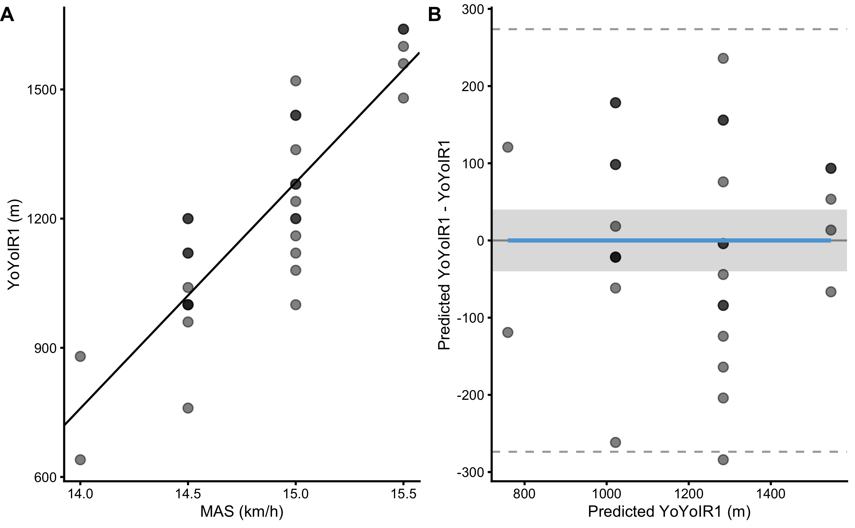
Figure 3.16: Scatter plot for simple linear regression between YoYoIR1 and MAS using the full training data sample. A. Scatter plot between YoYoIR1 and MAS scores. Black line indicates model prediction. B. Scatter plot between \(y_{predicted}\) (fitted or predicted YoYoIR1) against model residual \(y_{residual} = y_{predicted} - y_{observed}\), or Predicted YoYoIR1 - YoYoIR1. Dotted lines indicate Levels of Agreement (LOA; i.e. upper and lower threshold that contain 95% of residuals distribution) and grey band indicates SESOI. Blue line indicate linear regression fit of the residuals and is used to indicate issues with the model (residuals)

Predictive performance metrics can be found in the Table 3.10. As already expected, predicting YoYoIR1 from the MAS score, given the data collected, SESOI and linear regression model is not precise enough to be practically useful. Please note that the R-squared is very close to R-squared from the Table 3.10, but the PPER is much worse. Another reason to complement contemporary estimators with magnitude-based ones.

Table 3.11: Predictive performance summary

metric	training	training.pooled	testing.pooled	mean	SD	min	max
MBE	0.00	0.00	3.13	1.95	50.33	-96.20	82.14
MAE	104.69	103.04	112.98	112.59	24.99	66.61	154.76
RMSE	129.30	127.55	138.73	135.92	26.46	82.62	175.52
PPER	0.24	0.25	0.23	0.22	0.05	0.17	0.34
SESOI to RMSE	0.62	0.63	0.58	0.61	0.14	0.46	0.97
R-squared	0.74	0.74	0.70	0.70	0.14	0.48	0.88
MinErr	-235.93	-261.63	-253.04	-193.59	43.68	-253.04	-76.70
MaxErr	284.07	309.00	323.53	225.37	89.69	51.02	323.53
MaxAbsErr	284.07	309.00	323.53	260.89	44.88	158.47	323.53

In the second part of this book, we will get back to this example and estimate predictive performance using different models besides linear regression (like baseline prediction and regression trees)

References

7. Altmann, T, Bodensteiner, J, Dankers, C, Dassen, T, Fritz, N, Gruber, S, et al. Limitations of Interpretable Machine Learning Methods. 2019.

12. Barron, JT. A General and Adaptive Robust Loss Function. arXiv:170103077 [cs, stat], 2019.Available from: http://arxiv.org/abs/1701.03077

15. Biecek, P and Burzykowski, T. Predictive Models: Explore, Explain, and Debug. 2019.

25. Botchkarev, A. A New Typology Design of Performance Metrics to Measure Errors in Machine Learning Regression Algorithms. Interdisciplinary Journal of Information, Knowledge, and Management 14: 045–076, 2019.

26. Breheny, P and Burchett, W. Visualization of regression models using visreg. The R Journal 9: 56–71, 2017.

27. Breiman, L. Statistical Modeling: The Two Cultures. Statistical Science 16: 199–215, 2001.

31. Carsey, T and Harden, J. Monte Carlo Simulation and Resampling Methods for Social Science. 1 edition. Los Angeles: Sage Publications, Inc, 2013.

33. Chai, T and Draxler, RR. Root mean square error (RMSE) or mean absolute error (MAE)? Arguments against avoiding RMSE in the literature. Geoscientific Model Development 7: 1247–1250, 2014.

49. Fox, J. Effect displays in R for generalised linear models. Journal of Statistical Software 8: 1–27, 2003.Available from: http://www.jstatsoft.org/v08/i15/

51. Fox, J and Weisberg, S. Visualizing fit and lack of fit in complex regression models with predictor effect plots and partial residuals. Journal of Statistical Software 87: 1–27, 2018.Available from: https://www.jstatsoft.org/v087/i09

53. Friedman, J, Hastie, T, and Tibshirani, R. Regularization paths for generalized linear models via coordinate descent. Journal of Statistical Software 33: 1–22, 2010.

60. Goldstein, A, Kapelner, A, Bleich, J, and Pitkin, E. Peeking Inside the Black Box: Visualizing Statistical Learning with Plots of Individual Conditional Expectation. arXiv:13096392 [stat], 2013.Available from: http://arxiv.org/abs/1309.6392

61. Greenwell, B, Boehmke, B, and Gray, B. Vip: Variable importance plots. 2020.Available from: https://CRAN.R-project.org/package=vip

62. Greenwell, BM. Pdp: An r package for constructing partial dependence plots. The R Journal 9: 421–436, 2017.Available from: https://journal.r-project.org/archive/2017/RJ-2017-016/index.html

63. Greenwell, BM. Pdp: An R Package for Constructing Partial Dependence Plots. The R Journal 9: 421–436, 2017.

64. Hamner, B and Frasco, M. Metrics: Evaluation metrics for machine learning. 2018.Available from: https://CRAN.R-project.org/package=Metrics

73. Hernán, MA. Does water kill? A call for less casual causal inferences. Annals of epidemiology 26: 674–680, 2016.

76. Hernán, MA, Hsu, J, and Healy, B. A Second Chance to Get Causal Inference Right: A Classification of Data Science Tasks. CHANCE 32: 42–49, 2019.

77. Hernán, MA and Robins, J. Causal Inference. Boca Raton: Chapman & Hall/CRC,.

85. Hopkins, WG. Understanding Statistics by Using Spreadsheets to Generate and Analyze Samples. Sportscience.org., 2007.Available from: https://www.sportsci.org/2007/wghstats.htm

92. James, G, Witten, D, Hastie, T, and Tibshirani, R. An Introduction to Statistical Learning: With Applications in R. 1st ed. 2013, Corr. 7th printing 2017 edition. New York: Springer, 2017.

103. Kleinberg, J, Liang, A, and Mullainathan, S. The Theory is Predictive, but is it Complete? An Application to Human Perception of Randomness. arXiv:170606974 [cs, stat], 2017.Available from: http://arxiv.org/abs/1706.06974

104. Kleinberg, S. Causality, probability, and time. 2018.

105. Kleinberg, S. Why: A Guide to Finding and Using Causes. 1 edition. Beijing ; Boston: O’Reilly Media, 2015.

110. Kuhn, M and Johnson, K. Feature Engineering and Selection: A Practical Approach for Predictive Models. Milton: CRC Press LLC, 2019.

111. Kuhn, M and Johnson, K. Applied Predictive Modeling. 1st ed. 2013, Corr. 2nd printing 2016 edition. New York: Springer, 2018.

112. Kuhn, M, Wing, J, Weston, S, Williams, A, Keefer, C, Engelhardt, A, et al. Caret: Classification and Regression Training. 2018.

132. Miller, T. Explanation in Artificial Intelligence: Insights from the Social Sciences. arXiv:170607269 [cs], 2017.Available from: http://arxiv.org/abs/1706.07269

137. Molnar, C. Interpretable Machine Learning. Leanpub, 2018.

138. Molnar, C, Bischl, B, and Casalicchio, G. Iml: An R package for Interpretable Machine Learning. JOSS 3: 786, 2018.

147. Pearl, J. Causal inference in statistics: An overview. Statistics Surveys 3: 96–146, 2009.

148. Pearl, J. The seven tools of causal inference, with reflections on machine learning. Communications of the ACM 62: 54–60, 2019.

150. Pearl, J and Mackenzie, D. The Book of Why: The New Science of Cause and Effect. 1 edition. New York: Basic Books, 2018.

154. R Core Team. R: A language and environment for statistical computing. Vienna, Austria: R Foundation for Statistical Computing, 2020.Available from: https://www.R-project.org/

157. Ribeiro, MT, Singh, S, and Guestrin, C. "Why Should I Trust You?": Explaining the Predictions of Any Classifier. arXiv:160204938 [cs, stat], 2016.Available from: http://arxiv.org/abs/1602.04938

159. Rousselet, GA, Pernet, CR, and Wilcox, RR. A practical introduction to the bootstrap: A versatile method to make inferences by using data-driven simulations., 2019.

163. Saddiki, H and Balzer, LB. A Primer on Causality in Data Science. arXiv:180902408 [stat], 2018.Available from: http://arxiv.org/abs/1809.02408

177. Shmueli, G. To Explain or to Predict? Statistical Science 25: 289–310, 2010.

187. Watts, DJ, Beck, ED, Bienenstock, EJ, Bowers, J, Frank, A, Grubesic, A, et al. Explanation, prediction, and causality: Three sides of the same coin?, 2018.

203. Willmott, C and Matsuura, K. Advantages of the mean absolute error (MAE) over the root mean square error (RMSE) in assessing average model performance. Climate Research 30: 79–82, 2005.

206. Yarkoni, T and Westfall, J. Choosing Prediction Over Explanation in Psychology: Lessons From Machine Learning. Perspectives on Psychological Science 12: 1100–1122, 2017.

207. Zhao, Q and Hastie, T. Causal Interpretations of Black-Box Models. Journal of Business & Economic Statistics 1–10, 2019.

---

15. Some authors refer to causal inference as “explanatory” modeling (27,177,206), although Miguel Hernan warns against using such a somewhat-misleading term “because causal effects may be quantified while remaining unexplained (randomized trials identify causal effects even if the causal mechanisms that explain them are unknown)” (76). Andrew Gelman also makes distinctions between forward causal inference and reverse causal inference that might be useful in distinguishing between identifying causal effects and explaining them (54). This is elaborated in the Causal inference section of this book.↩︎

16. For example, if an athlete lifted 175kg for a single rep in the back squat, and was unable to lift more, this represents his back squat 1RM, or one repetition maximum. Relative 1RM is calculated by dividing 1RM with athlete’s bodyweight. For example, an athlete with 175kg 1RM weights 85kg. His relative 1RM is equal to 2.05.↩︎

17. Uncovering DGP parameters is not solely the goal of the causal inference (although causal inference task is to uncover or quantify causal mechanism), but also the main goal in the statistical inference where the aim is to quantify uncertainty about the true population parameters from the acquired sample. More about this topic in the Statistical Inference section.↩︎

18. As explained in Introduction section, I will mostly focus at variables on continuous ratio scale. Prediction error metrics differ for target variable that is on nominal scale (i.e. classification task) and involve estimators such as accuracy, specificity, sensitivity, area under curve (AUC) (111,118).↩︎

19. Although I’ve used the term loss here, these loss functions are also aggregated using sum or mean to create Huber cost or Ridge cost. Huber loss is a combination of absolute and quadratic losses and it’s property is better robustness to outliers.↩︎

20. MSE will be removed from the further analysis and tables since it is equivalent to RMSE, just squared.↩︎

21. As it will be explained in Statistical inference section, there are two kinds of uncertainty: aleatory and epistemic. Aleatory uncertainty is inherent randomness and it is usually represented as irreducible error. Epistemic uncertainty is due to the lack of knowledge or information, which can be considered reducible error. In other words, better models or models with more information will be able to reduce prediction error by reducing the reducible or epistemic uncertainty. The upper ceiling of the predictive performance is determined by irreducible error (which is unknown). Please refer to the Statistical inference section for more information.↩︎

22. Or to utilize subject matter knowledge needed to select the model. More about this topic can be found in the Subject matter knowledge section.↩︎

23. With the recent laws such as European’s DGPR, predictive models needs to be able to explain or provide explanation why particular decision or prediction has been made. Christoph Molnar explains the need for model interpretability with one interesting example: “By default, machine learning models pick up biases from the training data. This can turn your machine learning models into racists that discriminate against protected groups. Interpretability is a useful debugging tool for detecting bias in machine learning models. It might happen that the machine learning model’s, you have trained for, automatic approval or rejection of credit applications discriminates against a minority. Your main goal is to grant loans only to people who will eventually repay them. The incompleteness of the problem formulation in this case lies in the fact that you not only want to minimize loan defaults, but are also obliged not to discriminate on the basis of certain demographics. This is an additional constraint that is part of your problem formulation (granting loans in a low-risk and compliant way) that is not covered by the loss function the machine learning model was optimized for.” (137)↩︎

24. “Pearl’s causal meta-model involves a three-level abstraction he calls the ladder of causation. The lowest level, Association (seeing/observing), entails the sensing of regularities or patterns in the input data, expressed as correlations. The middle level, Intervention (doing), predicts the effects of deliberate actions, expressed as causal relationships. The highest level, Counterfactuals (imagining), involves constructing a theory of (part of) the world that explains why specific actions have specific effects and what happens in the absence of such actions” (197)↩︎

25. As you will learn in Statistical inference section, we can perform statistical tests (in this case t-test) to check whether the average of the cross-validated performance metric differ from metric estimated on the full training sample.↩︎