Chapter 10 Measurement Error

Measurement error is involved in all measurements and causes an observed score to be different from the true score (4,22,144,179). This results in measurement bias affecting descriptive analysis, causal inferences (72,74,77), and predictive performances (111).

In mathematical notation, observed score (OS) comprises of the hypothetical true score (TS) and measurement error (ME) (Equation (10.1)) (4,179). This conceptual model is called Classical Test Theory (for more information, philosophy, and issues behind it please see (22))

\[\begin{equation} OS = TS + ME \tag{10.1} \end{equation}\]

In the sports science domain, since the measured objects are usually humans, measurement error comprises of instrumentation and biological noise (179). In this book I assume instrumentation noise to be error caused solely by the measurement apparatus (179). Biological noise, on the other hand, is defined as an error in the observed scores caused by biological processes, including, but not limited to, phenomena such as circadian rhythm, nutritional intake, sleep and motivation (179). Thus, I prefer to use the terms instrumentation error and biological variation (these will be further discussed in the Extending the Classical Test Theory section)

Both instrumentation and biological noises consist of two types of errors: systematic error and random error (Figure 10.1)³⁴.

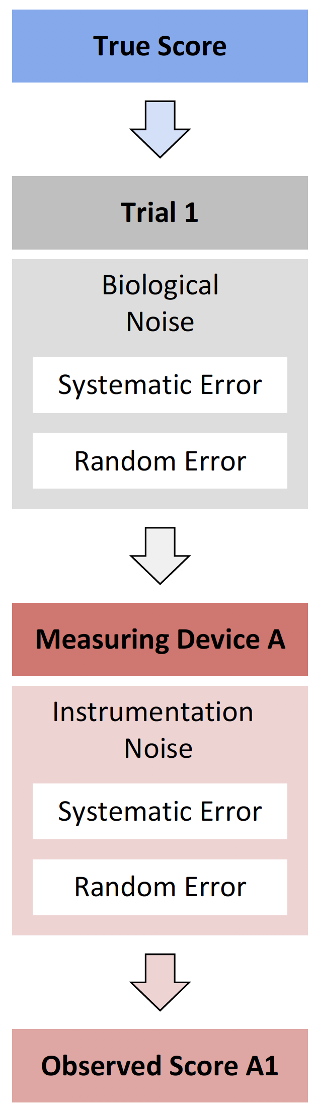
Figure 10.1: Measurement error components

Systematic error represents constant and stable error that is fixed across measurements. Systematic error is commonly refereed to as bias. With measurement instruments that have a linear response, systematic error can be further divided into proportional bias and fixed bias (84–86). Random error (\(\epsilon\)) represents unknown and unpredictable error, which varies between measurements. Random errors are often represented and modeled using a Gaussian normal distribution (with mean zero and SD which represent a parameter of the random error). The Equation (10.2) represent theoretical linear relationship between TS and OS, with normally distributed random error.

\[\begin{equation} OS = Fixed\; Bias + (Proportional \; Bias\times TS) + \epsilon \tag{10.2} \end{equation}\]

This can be easily explained with a simple example. Imagine N=20 athletes being measured on a novel bodyweight scale, using total of 5 trials separated by 1 minute. The assumption in this example is that there is no change in the TS across trials (e.g. athletes are not allowed to use bathroom, consume water or food, nor change the wardrobe) and that there is no biological noise involved (i.e. there are no fluctuations in bodyweight due motivation, fatigue or what have you). Since this is simulated example, we know the TS of the athletes, but also the instrumentation noise characteristic of the novel bodyweight scale (i.e. this represents the underlying DGP). This scale tends to have proportional bias equal to factor 1.01 (i.e. athlete weighting 100kg which is his TS, will have OS equal to 101kg due proportional bias, while the athlete weighting 50kg will have her OS equal to 50.5kg), fixed bias equal to 1kg (everyone will get OS higher for 1kg than TS), and random error normally distributed with SD equal to 0.5kg. Equation (10.3) captures this relationship between OS and TS.

\[\begin{equation} OS = 1 + (1.01 \times TS) + \mathcal{N}(0,\, 0.5) \tag{10.3} \end{equation}\]

Table 10.1 contains the simulated sample for N=20 athletes and 5 trials.

Table 10.1: Simulated 5 trials from known true score and measurement error

Athlete	TS (kg)	OS 1 (kg)	OS 2 (kg)	OS 3 (kg)	OS 4 (kg)	OS 5 (kg)
Athlete 01	77.93	79.47	79.37	79.25	80.38	79.46
Athlete 02	76.11	77.83	77.71	77.36	78.32	76.78
Athlete 03	77.04	78.65	78.30	78.48	78.30	78.55
Athlete 04	54.96	56.58	56.36	56.05	56.20	56.45
Athlete 05	84.03	85.53	85.44	86.10	85.96	85.11
Athlete 06	61.32	61.84	63.05	63.52	63.73	62.43
Athlete 07	68.62	70.26	69.82	70.34	70.45	70.84
Athlete 08	61.06	62.03	62.91	62.93	62.15	62.40
Athlete 09	80.46	81.34	83.04	82.57	82.60	82.33
Athlete 10	91.14	94.02	93.47	93.28	93.40	93.51
Athlete 11	79.98	81.89	82.13	81.13	81.57	81.94
Athlete 12	67.07	69.54	68.32	68.29	69.23	67.72
Athlete 13	79.41	80.66	80.81	81.17	80.56	80.92
Athlete 14	69.54	71.14	72.34	70.16	72.01	71.11
Athlete 15	76.01	77.42	77.41	78.32	78.22	77.61
Athlete 16	68.31	70.11	70.05	70.17	69.02	70.06
Athlete 17	58.53	60.04	60.56	59.69	59.72	60.69
Athlete 18	81.64	82.61	83.30	83.66	82.87	82.60
Athlete 19	55.03	56.70	56.35	56.90	56.48	56.37
Athlete 20	65.03	66.33	66.44	67.29	67.28	66.82

The objective of the analysis is to estimate DGP parameters of the measurement error (the proportional bias, fixed bias, and the SD of the random error). Unfortunately, since TS is unknown, we are unable to estimate proportional bias and fixed bias. To overcome this problem, we usually compare OS to some gold standard (or criterion) measure which can serve as proxy to TS. These issues are covered in much more detail in the second part of this book in the Validity and Reliability chapter.

What is left to be estimated is the SD of the random error, which is often referred to as typical error (TE) of the test, or standard error of the measurement (SEM)³⁵. TE is estimated using individual SD of the OS in the five trials (Table 10.2).

Table 10.2: Individual mean and SD from five trials

Athlete	Mean	SD
Athlete 01	79.59	0.45
Athlete 02	77.60	0.57
Athlete 03	78.46	0.16
Athlete 04	56.33	0.21
Athlete 05	85.63	0.40
Athlete 06	62.91	0.78
Athlete 07	70.34	0.37
Athlete 08	62.48	0.42
Athlete 09	82.38	0.63
Athlete 10	93.54	0.28
Athlete 11	81.73	0.39
Athlete 12	68.62	0.75
Athlete 13	80.82	0.24
Athlete 14	71.35	0.86
Athlete 15	77.80	0.44
Athlete 16	69.88	0.49
Athlete 17	60.14	0.47
Athlete 18	83.01	0.46
Athlete 19	56.56	0.24
Athlete 20	66.83	0.45

The mean of athletes’ typical errors (SD in Table 10.2) is equal to 0.45kg, which is quite close to DGP random error parameter of 0.5kg. The reason for the difference between estimated and true value of the random error SD is due to the sampling error, which is a topic covered in the Statistical inference section of this book.

Unfortunately, this method of estimating TE is not always practically feasible. TE is usually estimated with two trials (OS1 and OS2; see Table 10.3), by using SD of the difference scores (\(SD_{diff}\)) across athletes (83,179).

Table 10.3: Estimating Typical Error using SD of the difference scores

Athlete	OS 1 (kg)	OS 2 (kg)	Difference OS 2-1 (kg)
Athlete 01	79.47	79.37	-0.11
Athlete 02	77.83	77.71	-0.11
Athlete 03	78.65	78.30	-0.35
Athlete 04	56.58	56.36	-0.23
Athlete 05	85.53	85.44	-0.09
Athlete 06	61.84	63.05	1.22
Athlete 07	70.26	69.82	-0.44
Athlete 08	62.03	62.91	0.88
Athlete 09	81.34	83.04	1.70
Athlete 10	94.02	93.47	-0.55
Athlete 11	81.89	82.13	0.24
Athlete 12	69.54	68.32	-1.22
Athlete 13	80.66	80.81	0.15
Athlete 14	71.14	72.34	1.21
Athlete 15	77.42	77.41	-0.01
Athlete 16	70.11	70.05	-0.06
Athlete 17	60.04	60.56	0.52
Athlete 18	82.61	83.30	0.70
Athlete 19	56.70	56.35	-0.35
Athlete 20	66.33	66.44	0.11

If we calculate SD of the difference scores from the Table 10.3, we get 0.7kg. However, this is not quite right, since we know that the true SD of the random error is 0.5kg. This happens because random error is affecting both Trial 1 (OS1) and Trial 2 (OS2), and is propagated to the difference between the two (Figure measurement-error-propagation). This is exactly the same concept as described in the Example of randomized control trial. The benefit of using squared errors and assuming Gaussian error distribution, as alluded multiple times in this book, is that this propagation can be mathematically and neatly expressed and estimated.

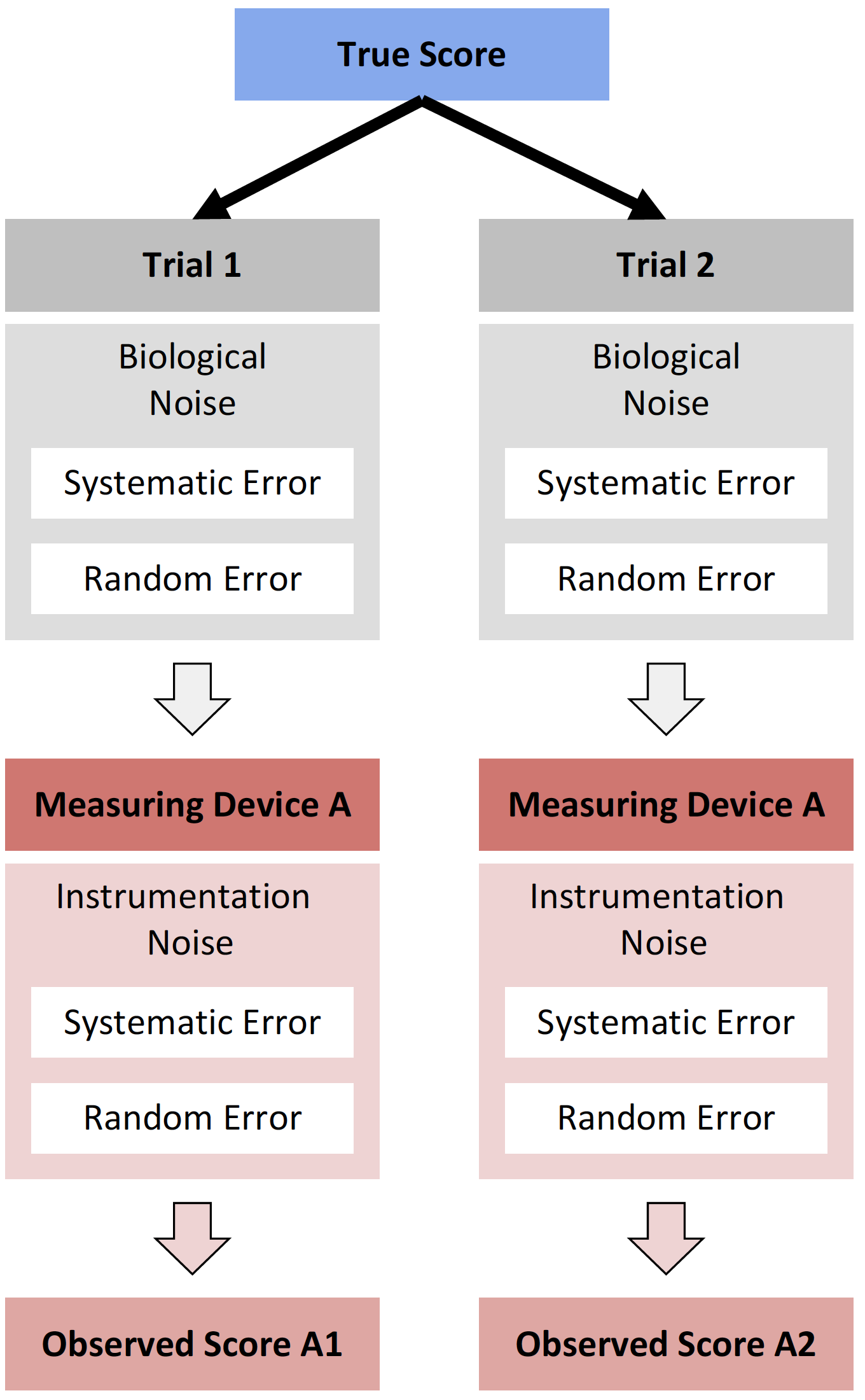
Figure 10.2: Propagation of the random component of measurement error to two trials

Error propagation, assuming normal distribution, is equal to Equation (10.4):

\[\begin{equation} \begin{split} SD_{difference}^2 &= TE_{trial\;1}^2 + TE_{trial\;2}^2 \\ TE_{test} &= TE_{trial\;1} = TE_{trial\;2} \\ SD_{difference}^2 &= TE_{test}^2 + TE_{test}^2 \\ SD_{difference}^2 &= 2 \times TE_{test}^2 \\ SD_{difference} &= \sqrt{2 \times TE_{test}^2} \\ SD_{difference} &= \sqrt{2} \times TE_{test} \\ TE_{test} &= \frac{SD_{difference}}{\sqrt{2}} \end{split} \tag{10.4} \end{equation}\]

According to the Equation (10.4), the SD of the difference score needs to be divided by \(\sqrt{2}\) to estimate TE of the measurement. The assumption is that TE is equal in both trials (and for all athletes), which is defined in the second line in the Equation (10.4). Estimated TE is now equal to 0.49kg, which is much closer to known SD of the random error of 0.5kg.

10.1 Estimating TE using ordinary least products regression

The method of estimating TE using SD of the difference score can be termed method of the differences and it is quite commonly used in Validity and Reliability analyses, particularly when using Bland-Altman plots. Another method involves the use of the linear regression, or the special kind of linear regression called ordinary least products (OLP) (121–124,140). The ordinary least squares (OLS; the one we have used thorough this book) regression find the line that minimizes squared residuals between \(y_i\) and \(\hat{y_i}\), while OLP minimizes the product of the residuals using both \(x\) and \(y\): \((x_i - \hat{x_i}) \times (y_i - \hat{y_i})\). The benefit of using OLP over OLS is that estimated model is the same regardless of which variable is considered outcome or predictor. This is not the case with OLS, as demonstrated in the Describing relationship between two variables section. For this reason, OLP is a preferred choice when performing Reliability analyses, since neither variable is considered outcome.

Figure 10.3 demonstrate OLP regression between Trial 1 (OS1) and Trial 2 (OS2). Estimated residual standard error (RSE) is equal to 0.72cm. To estimate TE, this RSE also needs to be divided by \(\sqrt{2}\), which results in 0.51cm. This estimate of TE is very close to TE estimated by the method of differences.

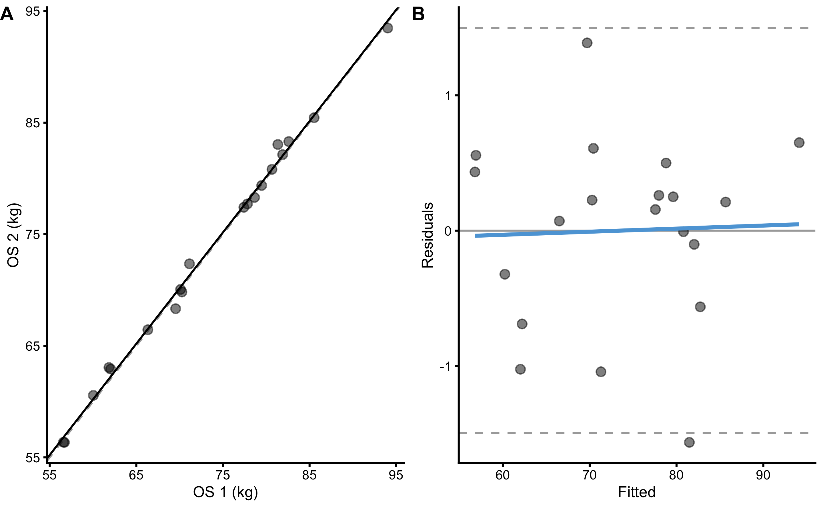
Figure 10.3: Ordinary least squares regression (OLP) between Trial 1 (OS1) and Trial 2 (OS2). A. Scatter-plot between OS1 and OS2. Dashed line represent identity line, and black line represent estimated OLP regression. B. Residuals plot. Dashed lines represent upper and lower levels of agreement using RSE and 95% confidence level (or in other words, 95% of the residuals distribution will be within these two dashed lines). Blue line represent additional linear regression model (using OLS) between fitted and residual, used to indicate issue with the model.

If we consider ±1kg to be SESOI in the observed score, we can estimate practical reliability of this scale. Magnitude-based estimators, such as PPER or SESOI to RSE can be used to quantify scale reliability from a practical significance perspective. This can be represented with the SESOI band as done in the Figure 10.4.

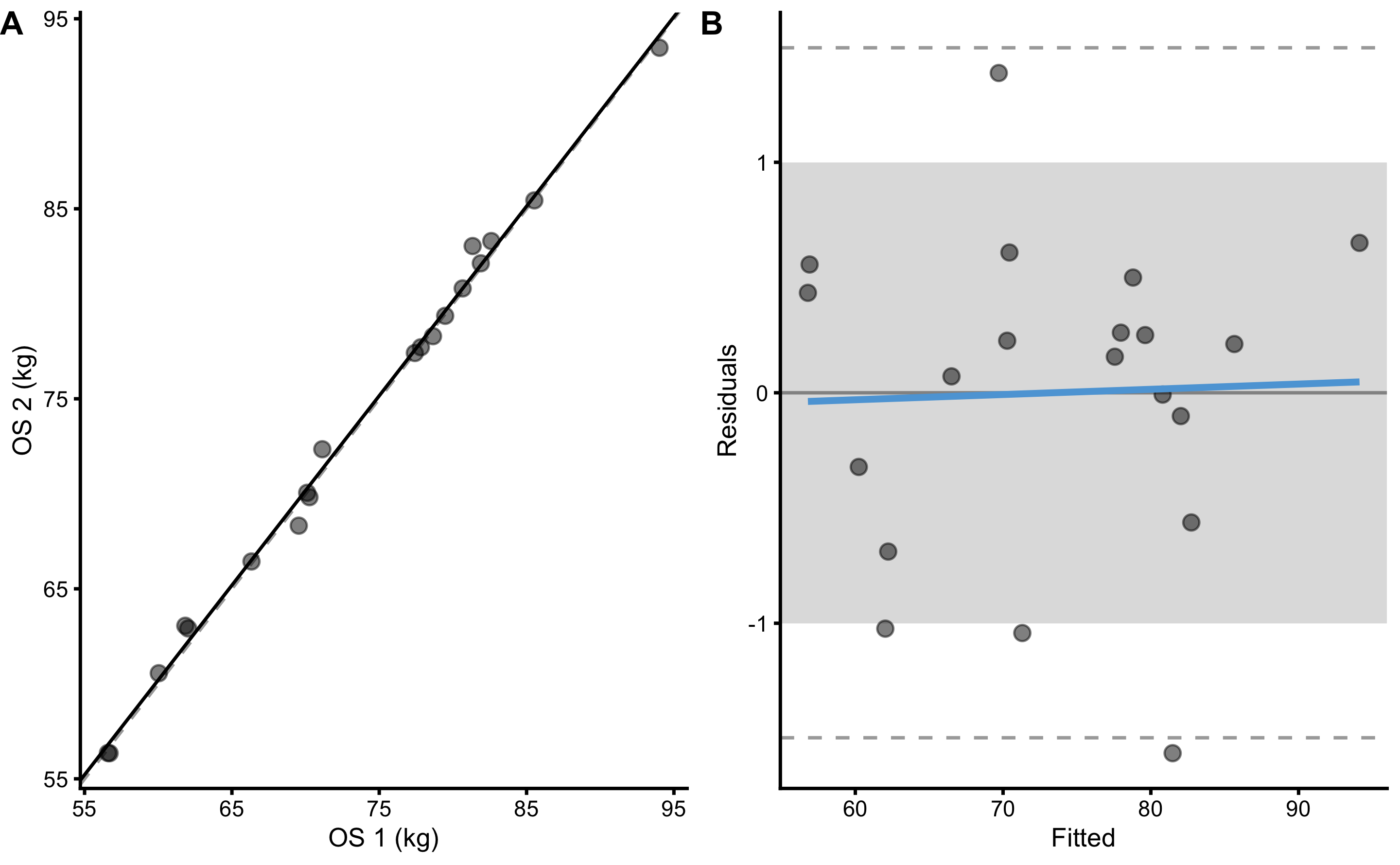
Figure 10.4: Ordinary least squares regression (OLP) between Trial 1 (OS1) and Trial 2 (OS2). A. Scatter-plot between OS1 and OS2. Dashed line represent identity line, and black line represent estimated OLP regression. B. Residuals plot. Dashed lines represent upper and lower levels of agreement using RSE and 95% confidence level (or in other words, 95% of the residuals distribution will be within these two dashed lines). Blue line represent additional linear regression model (using OLS) between fitted and residual, used to indicate issue with the model. SESOI is represented with the grey band. Residuals within SESOI band are of no practical difference. Proportion of residuals within SESOI band represent PPER estimator.

As can be seen from the Figure 10.4, this scale have less than perfect reliability to detect practically important changes in weight (given a priori defined SESOI of ±1kg). Estimated PPER, using RSE, is equal to 0.82.

10.2 Smallest Detectable Change

In the case of reliability and validity analysis, we are mostly interested in the ability of a measure to detect signal from a noise. In this case, the signal is the true or real change and noise is the random error of the measure. Thus, we are interested in estimating what is the smallest detectable signal the measure can detect with certain level of confidence. This is called smallest detectable change (SDC) or minimal detectable change (MDC).

If you check the Panel B in the Figure 10.4, SDC represents the spread of the residuals, visualized with the two horizontal dashed lines. If we assume that the residuals are normally distributed, we can estimate lower and upper thresholds that capture, for example 95% of the residuals distribution. This is done by multiplying \(SD_{diff}\) or RSE with appropriate critical value from a Student’s t-distribution (i.e. or simply with ±1.96). We thus get the Equation (10.5) that we can use to estimate SDC with 95% level of confidence³⁶.

\[\begin{equation} \begin{split} SDC &= SD_{diff} \times \pm1.96 \\ SDC &= RSE \times \pm1.96 \\ SDC &= TE \times \sqrt{2} \times \pm1.96 \\ \end{split} \tag{10.5} \end{equation}\]

Using OLP regression estimate RSE (equal to 0.72), and critical value to cover 95% of the Student’s t-distribution (DF=19) equal to ±2.09, SDC for our scale is equal to ±1.5kg. This implies that, with the 95% confidence, we are able to detect true signal (i.e. change in weight) as low as ±1.5kg. If SDC is lower than SESOI, reliability of the measure is (practically) perfect. This is not the case for our scale. We cannot use it to detect changes of ±1kg with satisficing level of confidence.

SDC can also be used as SESOI in some other analysis utilizing this scale. For example, if we use nutrition intervention RCT utilizing this scale as a measure, we can use ±1.5kg as SESOI (in the absence of better defined SESOI) since that is the the minimum detectable effect size.

10.3 Interpreting individual changes using SESOI and SDC

In order to showcase the interpretation of the individual changes by using SESOI and SDC (named observed outcome approach in Analysis of the individual residuals: responders vs non-responders section), let’s consider bench press example from the Comparing dependent groups (repeated in the Table 10.4).

Table 10.4: Individual Pre and Post scores, as well as Change in the bench press 1RM

Athlete	Pre-test (kg)	Post-test (kg)	Change (kg)
Athlete 01	111.80	121.42	9.62
Athlete 02	95.95	102.13	6.18
Athlete 03	105.87	125.56	19.69
Athlete 04	98.79	109.67	10.87
Athlete 05	95.81	108.11	12.30
Athlete 06	95.27	92.67	-2.60
Athlete 07	97.75	106.03	8.28
Athlete 08	106.50	109.51	3.01
Athlete 09	80.62	95.96	15.34
Athlete 10	100.40	94.30	-6.11
Athlete 11	82.71	78.91	-3.80
Athlete 12	102.89	93.98	-8.91
Athlete 13	91.34	105.21	13.87
Athlete 14	111.14	108.07	-3.07
Athlete 15	95.13	96.01	0.88
Athlete 16	109.12	112.12	3.00
Athlete 17	91.87	103.41	11.54
Athlete 18	92.16	103.93	11.77
Athlete 19	108.88	119.72	10.84
Athlete 20	97.94	95.91	-2.03

Before commencing this simple intervention, measurement error of the bench press 1RM test is estimated (using TE estimator), and is equal to 2.5kg (N=19). Practically, this means that due to the biological and instrumentation error, 1RM in the bench press would tend to vary normally distributed with TE equal to 2.5kg, given, of course, no real change in the strength (i.e. no change in TS). Expected SDC (with 95% confidence level) is thus equal to \(\sqrt{2}\times TE \times \pm2.09\) (±7.39kg). Please note that TE of the change score is equal to \(\sqrt{2}\times TE\), or (3.54kg).

For the sake of example, ±5kg can be considered minimal important change, which will be used as SESOI. Since both TE and SESOI are known, the objective of the analysis is to estimate probability that the observed individual change score is practically significant (i.e. lower, equivalent, or higher compared to SESOI). This is because individual true changes are not known, but only observed changes. Change TE tells how much of observed change randomly varies around the true change score. The question trying to be answered is: “how likely individual’s true change is within lower, equivalent, or higher SESOI range, given the known change TE?”

Panel A in the Figure 10.5 depicts individual Change scores probabilistically using the known change TE (3.54kg). Using the SESOI as equivalent change, we can estimate individual probability of lower, equivalent, and higher change. Panel B in the Figure 10.5 depicts individual change scores with error bars representing SDC. The numbers in brackets on Panel B in the Figure 10.5 represent estimated probabilities of the true change score being lower, equivalent, and higher compared to SESOI. To be more certain of individual changes, SDC needs to be smaller compared to SESOI. Ratio between SESOI and change TE can thus represent an estimate of the test sensitivity to detect practically meaningful changes (i.e. SESOI to RSE estimator). The smallest change that has at least 95% chance of being higher or lower than SESOI is equal to \(SESOI \pm SDC\), or ±12.39kg. Graphically, bench press 1RM change of ±12.39kg is the smallest change, where 95% confidence intervals do not touch the SESOI band. Please note that inference from MET is slightly different, since METs use single-tailed tests, thus the critical value will be smaller that 2.09 (it will be 1.73 for single-tailed 95% confidence). This implies that 95% confidence intervals (i.e. SDC) can slightly cross SESOI threshold and still be considered “Higher” or "Lower.

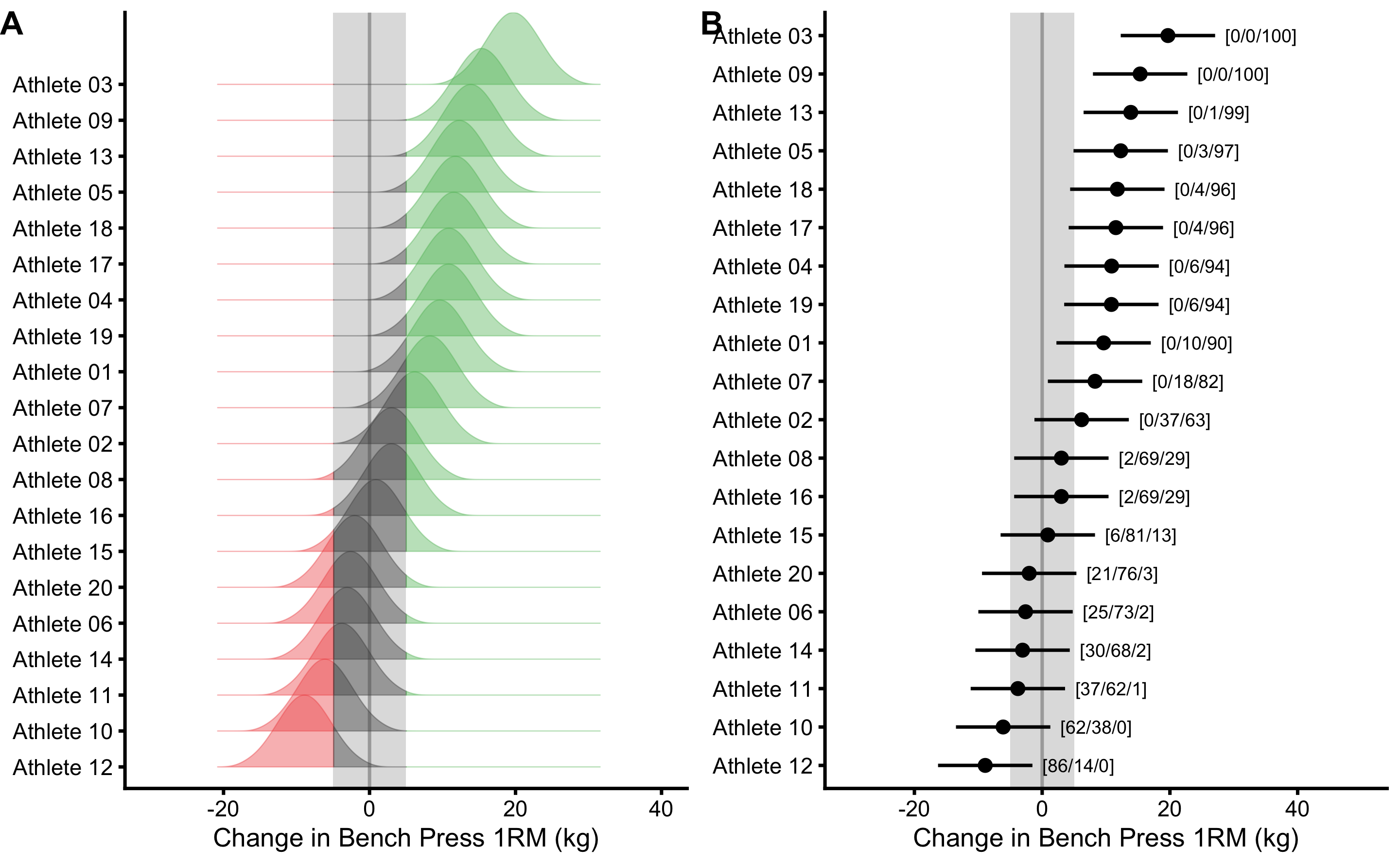
Figure 10.5: Analysis of individual change scores using SESOI and SDC. A. Uncertainty around true change score can be depicted by using normal distribution whose SD is equal to change TE. Probability that the observed change is lower, equivalent or higher can be estimated using surface within lower, equivalent, and higher magnitude band. B. \(95\%\) Confidence intervals around change scores represent SDC and are calculated using \(\pm 2.09\times\sqrt{2}\times TE\). Numbers in brackets represent proportion of the surface area in the lower, equivalent and higher magnitude band. These are interpreted as probabilities of true score being in lower, equivalent and higher magnitude band. See text for discussion why such interpretation is not statistically valid

As explained in the Statistical inference section of this book, this method of individual analysis interprets the change TE and associated confidence intervals from the Bayesian perspective. This is not the correct interpretation, since we do not know individual’s true change scores, only the observed change scores. Change TE gives us the variance of the observed change scores around the true change score, not vice versa (i.e. Bayesian inverse probability). Thus, visual representation from the Figure 10.5 is not statistically valid.

Since we do not know the true change scores, we are interested in probabilities of seeing the observed change score given the assumption of where we think the true change score is (i.e. null hypothesis). For this reason the question to be asked is “assuming individual’s true change scores are at ±SESOI, how likely are we to see the observed change score, given the known change TE?”. This question demands answer and interpretation of change TE from the frequentist perspective. Thus the correct interpretation of the individual changes involves the use of minimum effect tests (METs) discussed in the Statistical Inference section. METs approach to interpreting individual changes is depicted in the Figure 10.6.

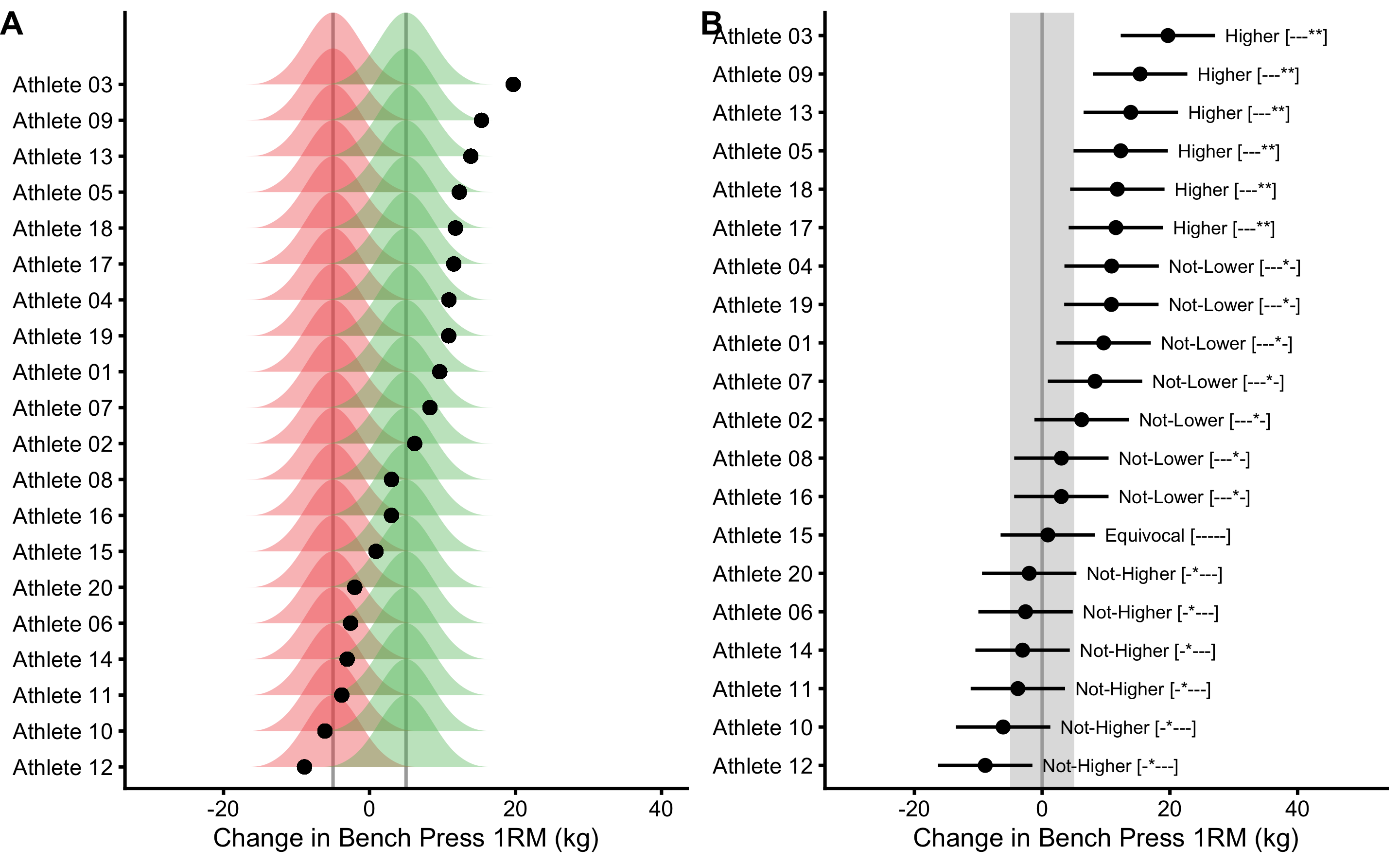
Figure 10.6: METs approach to interpreting individual change scores. A. Since true change scores are unknown, we can only test probability of seeing observed score or higher, given the known TE and assumed true score. In order to do this, minimal effect tests are performed, assuming two true score null-hypotheses: one at lower SESOI threshold (red color) and one at upper SESOI threshold (green color). Typical error can be interpreted as SD of the error distribution. Black dots indicate observed individual change. We are interested in estimating probability of observing this change, given two hypotheses. Five tests are performed as described in Minimum Effect Tests section: inferiority, non-superiority, equivalence, non-inferiority and superiority. B. \(95\%\) Confidence intervals around change scores represent SDC and are calculated using \(\pm 2.09\times\sqrt{2}\times TE\) and depicted using error-bars. Final inference using five METs is reported. METs significance (assuming alpha=0.05), indicated by ’*’, are reported in the brackets, for each of the the five tests performed

10.4 What to do when we know the error?

Statistical analysis covered in this book treats observed scores as true scores without measurement error. But measurement error is always involved and can introduce bias in the conclusion. How certain estimators and analyses are sensitive to measurement error can be estimated via simulations. But what can we do when we do know that there is measurement error involved in our observations and we actually have an estimate about it’s size (i.e. from validity or reliability study)?

There are few adjustment techniques that can be implemented (101,120,175,176,186), but here I will introduce Simulation extrapolation (SIMEX) approach since it is very intuitive. Let’s take the bench press example we used above: we do know that measurement error of 2.5kg is involved in the observed Pre- and Post-tests. How can we correct or adjust our estimators using that knowledge?

Since we know that error is already inside our observations, we can call that error factor or error multiplier of 1. Then we add additional error to our observations and repeat the analysis. This is done for error multipliers from 1 to usually 3 (i.e. extra 2 x measurement error). Let’s do that using bench press data and calculate mean and SD of the Pre-test, Post-test, and Change. This single simulation is in Figure 10.7.

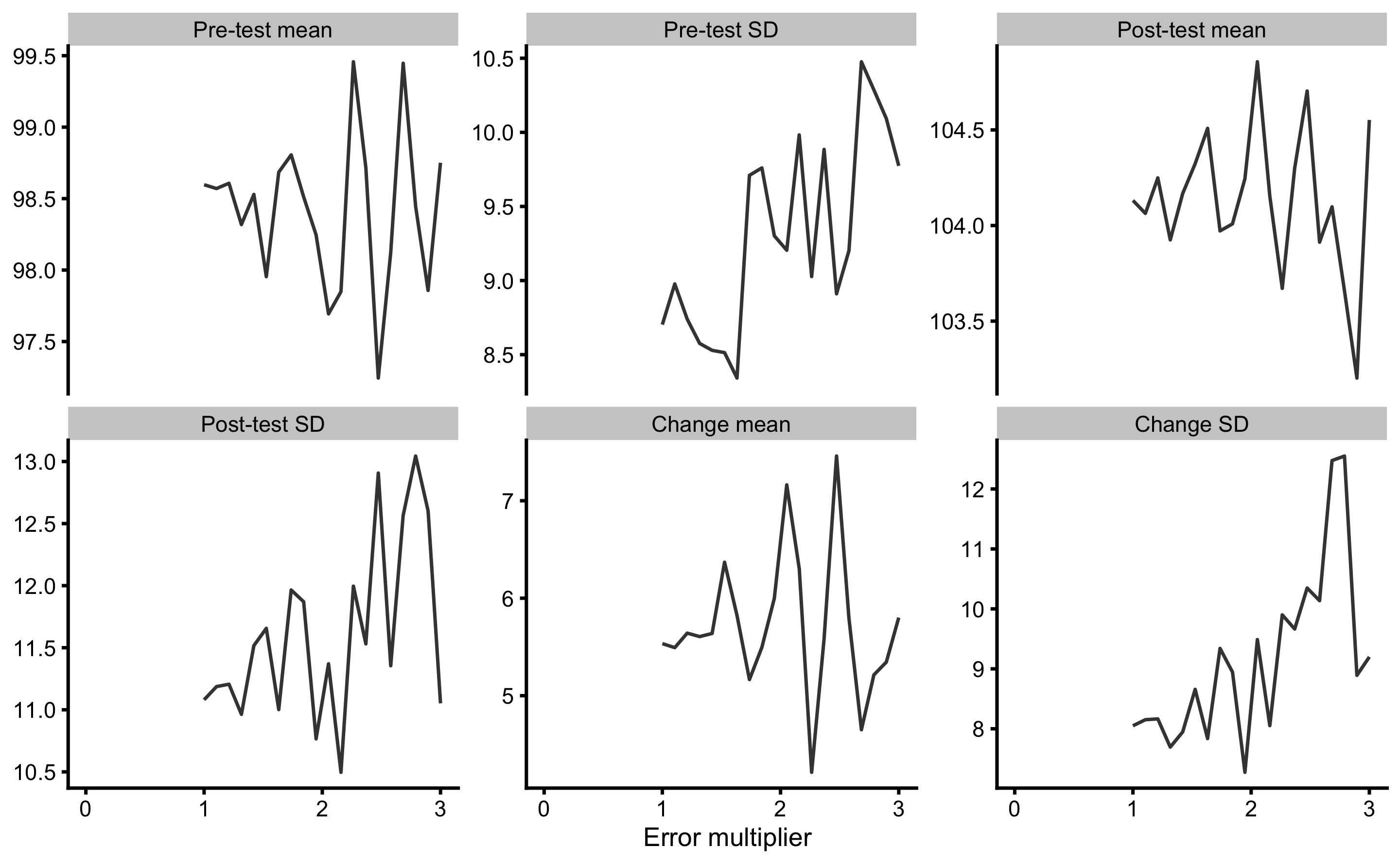
Figure 10.7: Adding noise (measurement error) to observed Pre-test and Post-test scores and re-calculating estimators. Error multiplier equal to 1 is naive analysis where one magnitude of measurement error (i.e. 2.5kg) is already involved in observed data. Additional error is added using error multiplier (i.e. error multiplier 2 involves additional noise of 2.5 kg magnitude, thus 2 error magnitudes are involved in the data) from 1 to 3, using total of 20 steps

We can’t conclude much since adding error multiplier once is stochastic. We need to repeat this numerous times, say 100 times. This is depicted in Figure 10.8.

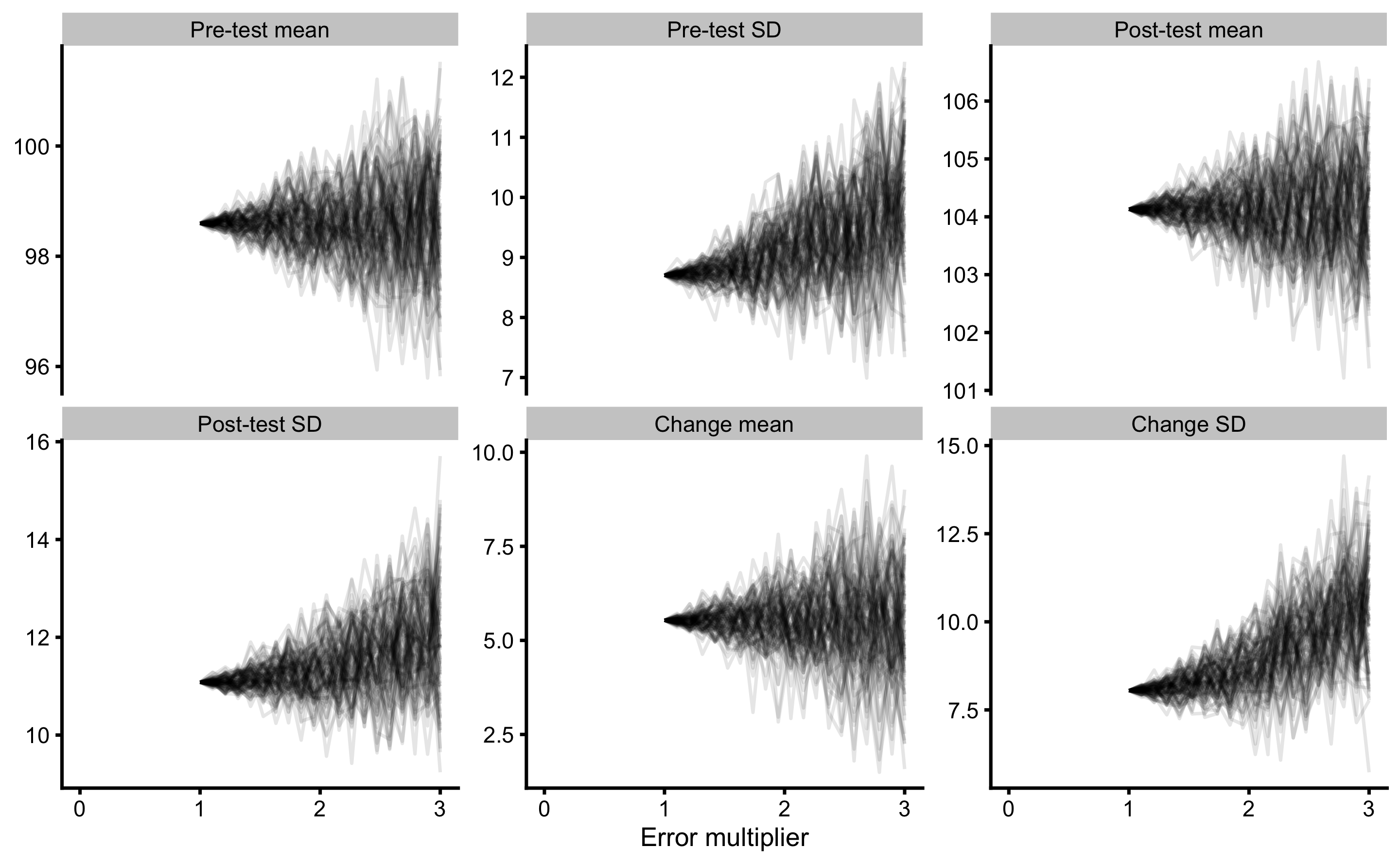
Figure 10.8: Result of SIMEX using 100 simulations

What we are interested in, is calculating the average or expected estimator value for each error multiplier. This is depicted in Figure 10.9

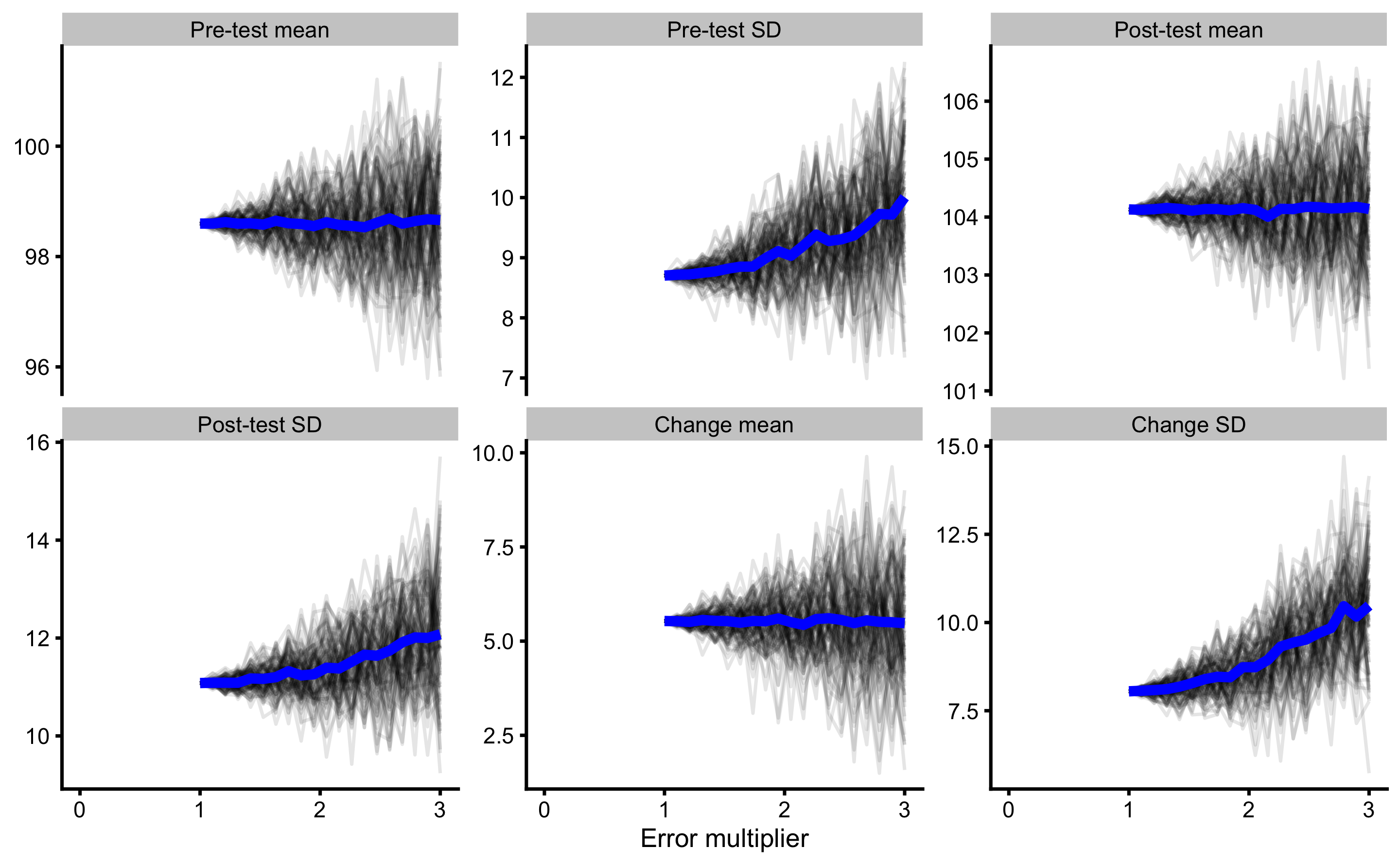
Figure 10.9: Result of SIMEX using 100 simulations and addition simulation average. Blue line represents simulations average for a particular error multiplier

Rather than using average across simulations, we can fit a particular model and then extrapolate to error multiplier of 0. This way we can get estimated estimator value when there is no measurement error involved in Pre-test and Post-test variables. Usually this is done using second order polynomial (i.e. \(\hat{y_i} = \beta_0 + \beta_1x_i + \beta_2x_i^2\)), or quadratic equation (i.e. \(\hat{y_i} = \beta_0 + \beta_1x_i^2\)). Extrapolating using quadratic equation is depicted in the Figure 10.10.

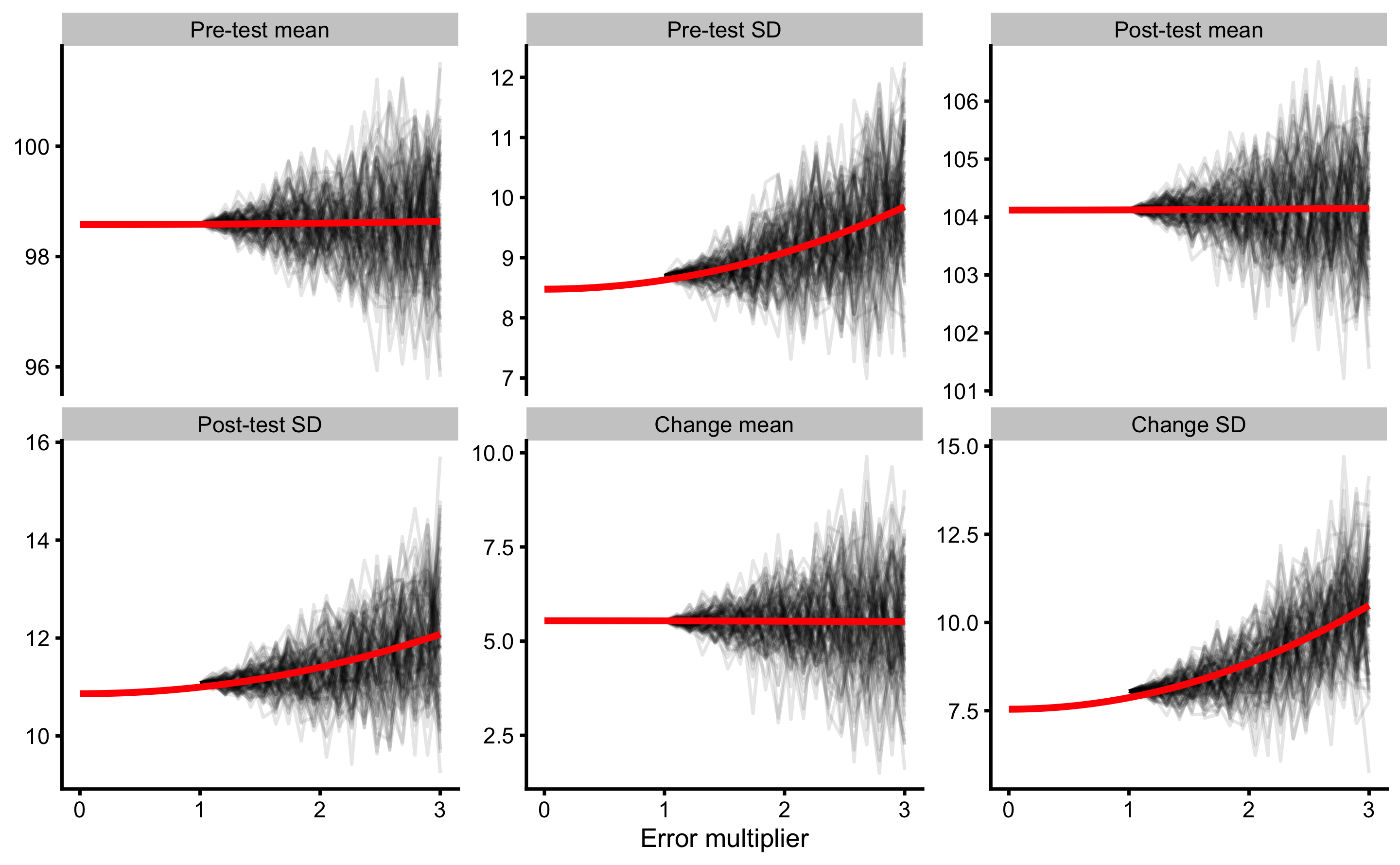
Figure 10.10: Result of SIMEX using 100 simulations and addition quadratic extrapolation. Red line represents quadratic fit, extrapolated to error multiplier of 0 to estimate estimator value when there is no measurement error involved in the Pre-test and Post-test variables

From 10.10 it is interesting to notice that mean is robust to measurement error, while SD is not, which is expected since normal error increase variance of the data. Using SIMEX for Change SD, we can estimate true Change SD, or in other words, when there is no measurement error. This can also be done using math rather than simulation and extrapolation (i.e. SIMEX) by using the same error propagation reasoning explained in the Example of randomized control trial section (Equation (10.6)).

\[\begin{equation} \begin{split} \sigma_{OS}^2 &= \sigma_{TS}^2 + \epsilon^2 \\ SD_{observed \; diff}^2 &= SD_{true \; diff}^2 + (\sqrt{2}TE)^2 \\ SD_{true \; diff} &= \sqrt{SD_{observed \; diff}^2 - 2TE^2} \end{split} \tag{10.6} \end{equation}\]

Observed Change SD is equal to 8.05kg, while the change TE is equal to \(\sqrt{2} \times 2.5\)kg or 3.53kg. True Change SD is thus equal to \(\sqrt{8.05^2 - 3.53^2 }\), or 7.23kg. This is also done when estimating stochastic treatment effect in the RCT, if we assume that the Change SD in the Control group is mainly due to measurement error.

10.5 Extending the Classical Test Theory

The theory behind true, observed scores, and measurement error introduced in this chapter is called Classical Test Theory (22). Although it sounds simple, there are numerous assumptions and issues with it (22):

"Classical test theory was either one of the best ideas in twentieth-century psychology, or one of the worst mistakes. The theory is mathematically elegant and conceptually simple, and in terms of its acceptance by psychologists, it is a psychometric success story. However, as is typical of popular statistical procedures, classical test theory is prone to misinterpretation. One reason for this is the terminology used: if a competition for the misnomer of the century existed, the term ‘true score’ would be a serious contestant. The infelicitous use of the adjective ‘true’ invites the mistaken idea that the true score on a test must somehow be identical to the ‘real’, ‘valid’, or ‘construct’ score. This chapter has hopefully proved the inadequacy of this view beyond reasonable doubt.

The problems with the platonic true score interpretation were, however, seen to run deeper than a confounding of validity and unreliability. Classical test theory is, ontologically speaking, ambiguous. In principle, it allows for both realist and constructivist interpretations, but sits well with neither. The constructivist interpretation of classical test theory is vacuous: although it is possible to specify how a true score could be constructed on the basis of observations (namely by averaging), the observations that are necessary for doing this are exactly the repeated measurements with intermediate brainwashing. The constructivist account of true scores can only be interpreted metaphorically, and it is not at all clear what such a metaphorical interpretation adds to the theory. On the other hand, a realist i terpretation of true scores leads to a metaphysical explosion of reality: a new true score has to be invoked for every thinkable testing procedure."

Let’s take the bench press example yet again. What is individual’s true score? Something that one can manifest? What if I have bench pressed 150kg, but got a flu and was off for 3 weeks. When I came back, I was able to bench press 130kg. Is my true bench press still 150kg, but masked due to systematic effect of the illness? What if this happens in a reliability study, and few individuals demonstrate true systematic effects of fatigue, while some demonstrate biological variability from day to day? We do assume Ergodicity in this example.

Figure 10.11 depicts my extension of the Classical Test Theory with performance specialist or sports scientist in mind (99). As alluded multiple time thorough this book, all statistical models represent “Small Worlds”, or simplifications of the complex “Large World” we ought to understand and interact with.

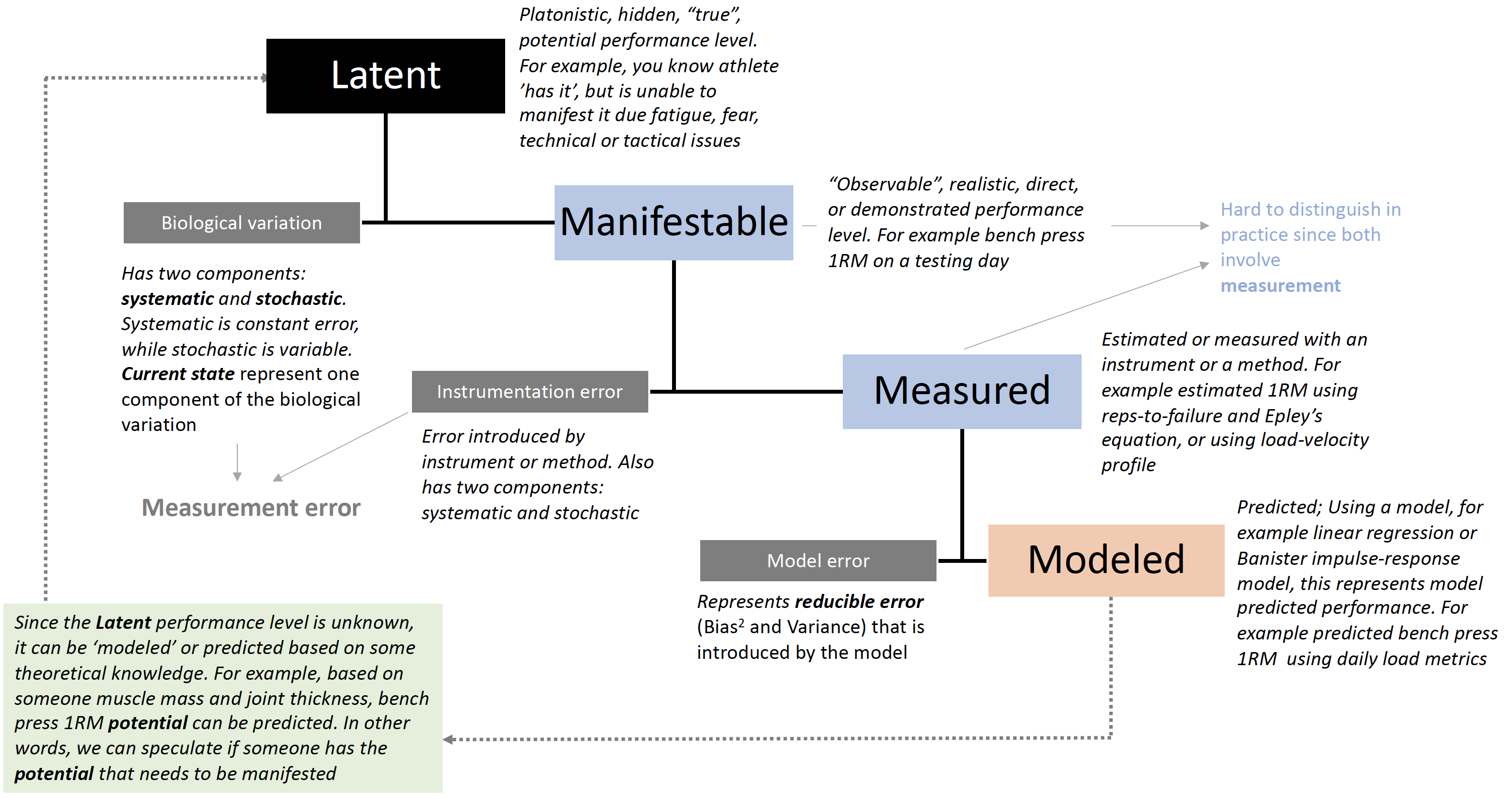
Figure 10.11: Circular Performance Model. Extended Classical Test Theory to include phenomenology of working with athletes

Circular Performance Model depicted in the Figure 10.11 (99) can be used to model and understand phenomena that sport practitioners and sports scientists wrestle with daily.

References

4. Allen, MJ and Yen, WM. Introduction to Measurement Theory. 1 edition. Long Grove, Ill: Waveland Pr Inc, 2001.

22. Borsboom, D. Measuring the mind: Conceptual issues in modern psychometrics. Cambridge: Cambridge University Press, 2009.

72. Hernan, MA and Cole, SR. Invited Commentary: Causal Diagrams and Measurement Bias. American Journal of Epidemiology 170: 959–962, 2009.

74. Hernán, MA. Causal Diagrams: Draw Your Assumptions Before Your Conclusions Course | PH559x | edX. edX., 2017.Available from: https://courses.edx.org/courses/course-v1:HarvardX+PH559x+3T2017/course/

77. Hernán, MA and Robins, J. Causal Inference. Boca Raton: Chapman & Hall/CRC,.

83. Hopkins, WG. Measures of Reliability in Sports Medicine and Science. Sports Med 15, 2000.

84. Hopkins, WG. Bias in Bland-Altman but not Regression Validity Analyses. Sportscience.org., 2004.Available from: https://sportsci.org/jour/04/wghbias.htm

86. Hopkins, WG. A Socratic Dialogue on Comparison of Measures. Sportscience.org., 2010.Available from: http://www.sportsci.org/2010/wghmeasures.htm

99. Jovanović, M. Extending the Classical Test Theory with Circular Performance Model. Complementary Training., 2020.

101. Keogh, RH, Shaw, PA, Gustafson, P, Carroll, RJ, Deffner, V, Dodd, KW, et al. STRATOS guidance document on measurement error and misclassification of variables in observational epidemiology: Part 1-Basic theory and simple methods of adjustment. Statistics in Medicine, 2020.

111. Kuhn, M and Johnson, K. Applied Predictive Modeling. 1st ed. 2013, Corr. 2nd printing 2016 edition. New York: Springer, 2018.

120. Lederer, W and Küchenhoff, H. A short introduction to the SIMEX and MCSIMEX. R News 6, 2006.

121. Ludbrook, J. SPECIAL ARTICLE COMPARING METHODS OF MEASUREMENT. Clinical and Experimental Pharmacology and Physiology 24: 193–203, 1997.

124. Ludbrook, J. A primer for biomedical scientists on how to execute Model II linear regression analysis: Model II linear regression analysis. Clinical and Experimental Pharmacology and Physiology 39: 329–335, 2012.

140. Mullineaux, DR, Barnes, CA, and Batterham, AM. Assessment of Bias in Comparing Measurements: A Reliability Example. Measurement in Physical Education and Exercise Science 3: 195–205, 1999.

144. Novick, MR. The axioms and principal results of classical test theory. Journal of Mathematical Psychology 3: 1–18, 1966.

175. Shang, Y. Measurement Error Adjustment Using the SIMEX Method: An Application to Student Growth Percentiles: Measurement Error Adjustment Using the SIMEX Method. Journal of Educational Measurement 49: 446–465, 2012.

176. Shaw, PA, Gustafson, P, Carroll, RJ, Deffner, V, Dodd, KW, Keogh, RH, et al. STRATOS guidance document on measurement error and misclassification of variables in observational epidemiology: Part 2-More complex methods of adjustment and advanced topics. Statistics in Medicine, 2020.

179. Swinton, PA, Hemingway, BS, Saunders, B, Gualano, B, and Dolan, E. A Statistical Framework to Interpret Individual Response to Intervention: Paving the Way for Personalized Nutrition and Exercise Prescription. Frontiers in Nutrition 5, 2018.

186. Wallace, M. Analysis in an imperfect world. Significance 17: 14–19, 2020.

---

34. These two types of error are conceptually equivalent to the bias and variance (see Prediction section), and systematic and stochastic intervention effects (see Causal inference section)↩︎

35. Both SEM and TE are used in the sports science literature and research. I personally prefer the simple random error, followed by TE. SEM has the same meaning as the standard error of the mean explained in the Frequentist perspective chapter and might create confusion.↩︎

36. This should also be done with TE if we want to quantify uncertainty around single observation with a particular level of confidence (e.g. multiply TE with ±1.96 to get 95% confidence), assuming normally distributed random error that is additive.↩︎