Simulation in vjsim
Mladen Jovanović
2020-08-04
Source:vignettes/simulation-vjsim.Rmd
simulation-vjsim.RmdSimulation
# Install vjsim if you haven't already by running the following commands
# install.packages("devtools")
# devtools::install_github("mladenjovanovic/vjsim")

# Install tidyverse and cowplot packages
# install.packages(c("tidyverse", "cowplot", "DT), dependencies = TRUE)

library(vjsim)
library(tidyverse)
library(cowplot)
library(DT)
Before reading this vignette, please read Introduction to vjsim vignette by running:
vignette("introduction-vjsim")
Basics of Newtonian mechanics
Now that we have explained the Force Generator characteristics and system constraints (i.e. mass, weight, push-off distance available), we can get into the simulation. Simply, Force Generator generates the ground reaction force (\(F_{GRF}\)) that acts on the object and produces acceleration (\(a\)). Since gravity acts on the object of mass \(m\), Force Generator needs to overcome both inertia (or mass \(m\)) and weight (which is the force in the opposite direction). The weight of the object is equal to \(weight = m \times 9.81\). If we put all of this into equation, we get the following:
\[ \begin{aligned} a &= \frac{F_{GRF}-w}{m} \\ a &= \frac{F_{GRF} - m\times 9.81}{m} \end{aligned} \] In the above equation \(F_{GRF} - m\times g\) represents net force, or propulsive force that is imposing acceleration on the object. Acceleration multiplied by change in time (\(dt\)) will yield change in velocity (\(dv\)):
\[ dv = a \times dt \]
Velocity multiplied by change in time (\(dt\)) will yield change in position (\(dd\)):
\[ dd = v \times dt \]
Let’s take an example. We have an object of mass 10kg that yields a weight of \(10 \times 9.81 = 98.1N\). The upward force of 1,000N is acting on this object. The net (propulsive force) is thus equal to:
\[ \begin{aligned} F_{net} &= 1000 - 98.1 \\ F_{net} & = 901.9N \end{aligned} \]
This net force acting on an object of mass 10kg will create acceleration equal to:
\[ \begin{aligned} a &= \frac{F_{net}}{m} \\ a &= \frac{901.9}{10} \\ a &= 90.19 ms^{-2} \end{aligned} \]
We are interested in what will happen to velocity and distance if this force of 1,000N is acting on the object of a mass of 10kg for 10second? We need to make a few assumptions. We assume that the initial velocity (\(v_0\)), initial position (distance) (\(d_0\)), and initial time (\(t_0\)) are all equal to zero.
Let’s start with plotting what we know about this problem:
kinetics_data <- tibble(
  GRF = 1000, # Ground reaction force; in Newtons
  mass = 10, # kg
  gravity_const = 9.81, # For Earth
  weight = mass * gravity_const, # In Newtons
  propulsive_force = GRF - weight,
  acceleration = propulsive_force / mass,
  time = seq(0, 10, length.out = 100)
)

plot_data <- gather(kinetics_data, "variable", "value", -time) %>%
  mutate(variable = factor(variable, levels = c(
    "GRF",
    "mass",
    "gravity_const",
    "weight",
    "propulsive_force",
    "acceleration"
  )))

ggplot(plot_data, aes(x = time, y = value)) +
  theme_cowplot(8) +
  geom_line(color = "blue") +
  facet_wrap(~variable, scales = "free_y") +
  ylab(NULL)
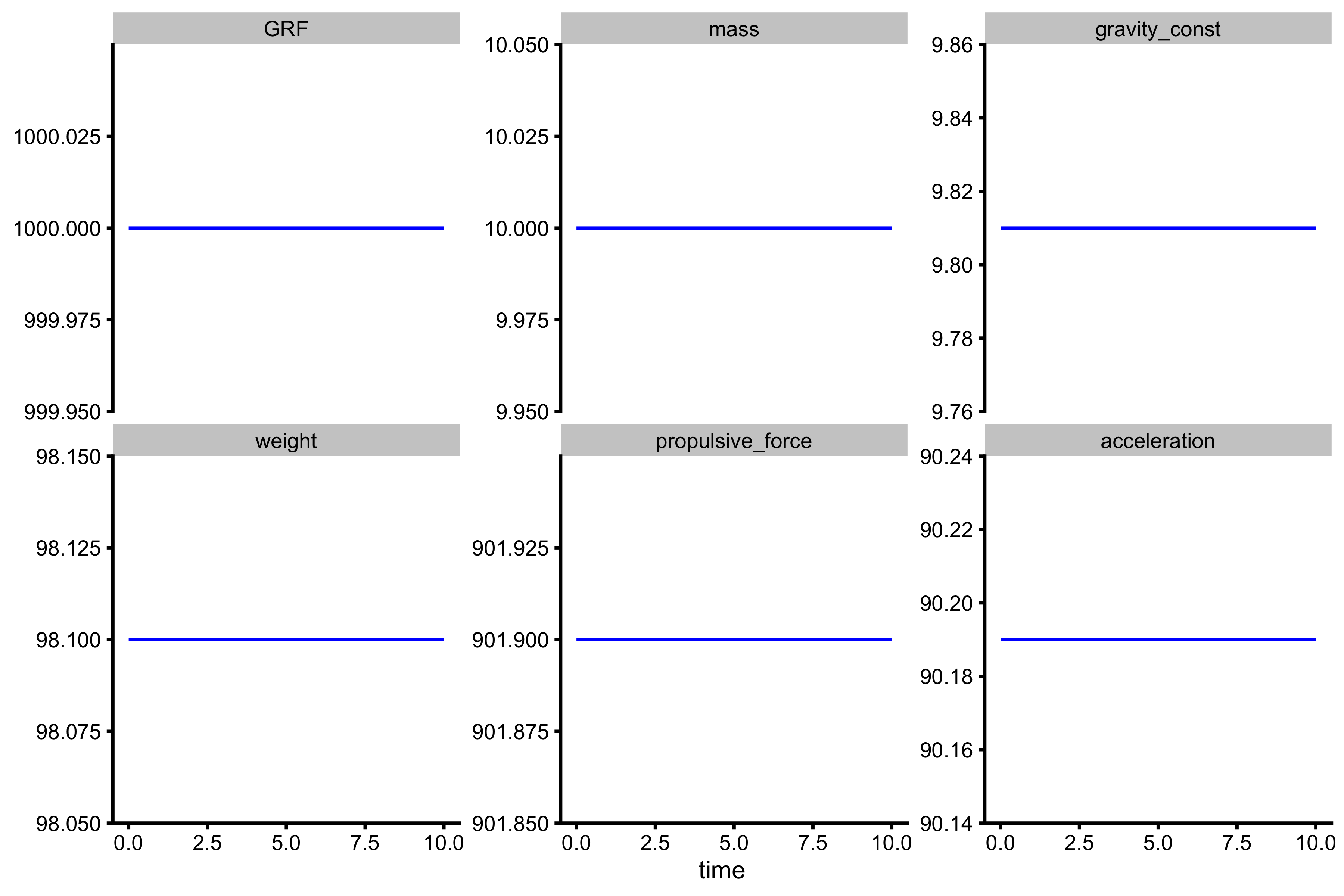
For this example we have used 1,000 points to represent change in time (from 0s to 10s), which is equal to \(dt = 0.01s\). Please note that this problem can be easily solved algebraically, but I will utilize Euler method to solve it, since it will be more intuitive to understand how does vjsim works.
So, if the body is accelerating for 0.01sec at the rate of \(90.19 ms^{-2}\), it means that the change in velocity (\(dv\)), assuming constant acceleration, will be equal to \(dv = 90.19 \times 0.01\), or 0.9019 \(ms^-1\). As stated, our initial velocity \(v_0\) (at \(t=0\)) is equal to zero, at \(t=0.01\), the velocity will be equal to:
\[ \begin{aligned} v_{t=0.01} &= v_{t=0} + dv \\ v_{t=0.01} &= 0 + 0.9019 \\ v_{t=0.01} &= 0.9019ms^-1 \end{aligned} \] For the next step we can repeat this iterative procedure. Hence for \(v_{t=0.02}\) the calculus is the following:
\[ \begin{aligned} v_{t=0.02} &= v_{t=0.01} + dv \\ v_{t=0.02} &= 0.9019 + 0.9019\\ v_{t=0.02} &= 1.8038ms^-1 \end{aligned} \]
We can do this in R:
velocity_0 <- 0 # Initial velocity
time_step <- 0.01

# Init the column in data frame
kinetics_data$velocity <- NA

# Save the initial velocity
kinetics_data$velocity[1] <- velocity_0

for (i in seq(1, nrow(kinetics_data) - 1)) {
  velocity_current <- kinetics_data$velocity[i]
  acceleration_current <- kinetics_data$acceleration[i]

  velocity_next <- velocity_current + acceleration_current * time_step

  # Save the next velocity
  kinetics_data$velocity[i + 1] <- velocity_next
}
If we plot this we will get the following:
plot_data <- gather(kinetics_data, "variable", "value", -time) %>%
  mutate(variable = factor(variable, levels = c(
    "GRF",
    "mass",
    "gravity_const",
    "weight",
    "propulsive_force",
    "acceleration",
    "velocity"
  )))

ggplot(plot_data, aes(x = time, y = value)) +
  theme_cowplot(8) +
  geom_line(color = "blue") +
  facet_wrap(~variable, scales = "free_y") +
  ylab(NULL)
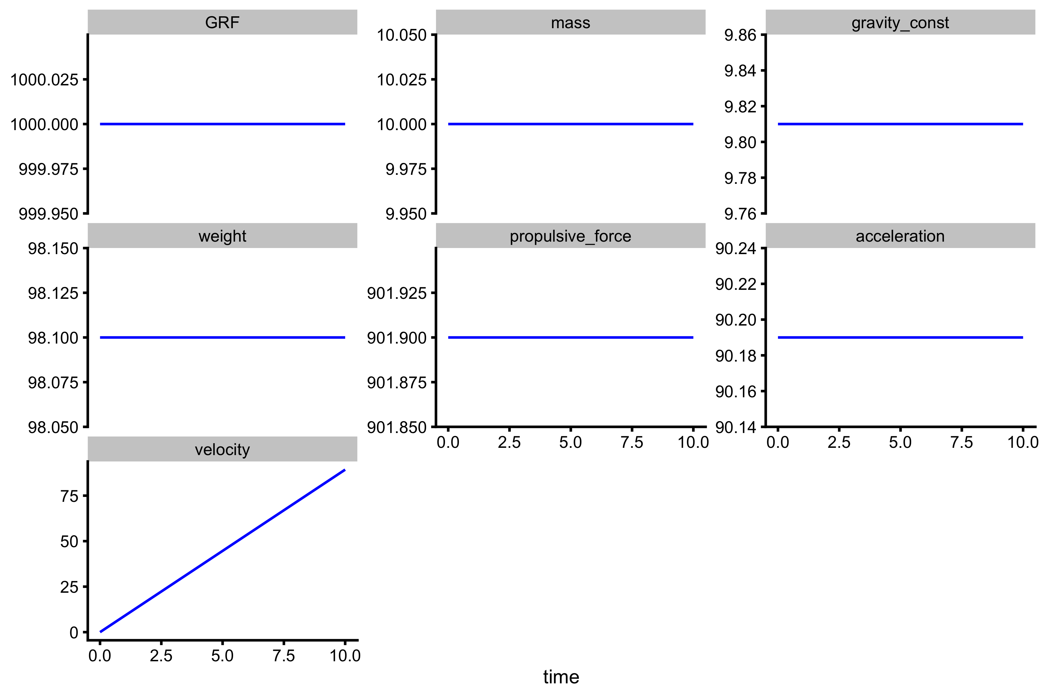
As can be seen, velocity is increasing due to constant acceleration. Rather than doing this by foot with iterations, we could simply write the equation for velocity:
\[ v_{t} = v_{0} + a \times t \] Ok, but what about distance traveled? As stated, the change in distance depends on velocity (\(dd = v \times dt\)). Assuming \(d_0\) is equal to 0, and time step equal to 0.01s, let’s repeat the same algorithm we have used for calculating velocity, but this time applies it for calculating distance:
distance_0 <- 0 # Initial distance
time_step <- 0.01

# Init the column in data frame
kinetics_data$distance <- NA

# Save the initial velocity
kinetics_data$distance[1] <- distance_0

for (i in seq(1, nrow(kinetics_data) - 1)) {
  distance_current <- kinetics_data$distance[i]
  velocity_current <- kinetics_data$velocity[i]

  distance_next <- distance_current + velocity_current * time_step

  # Save the next distance
  kinetics_data$distance[i + 1] <- distance_next
}
If we plot distance we will get the following:
plot_data <- gather(kinetics_data, "variable", "value", -time) %>%
  mutate(variable = factor(variable, levels = c(
    "GRF",
    "mass",
    "gravity_const",
    "weight",
    "propulsive_force",
    "acceleration",
    "velocity",
    "distance"
  )))

ggplot(plot_data, aes(x = time, y = value)) +
  theme_cowplot(8) +
  geom_line(color = "blue") +
  facet_wrap(~variable, scales = "free_y") +
  ylab(NULL)
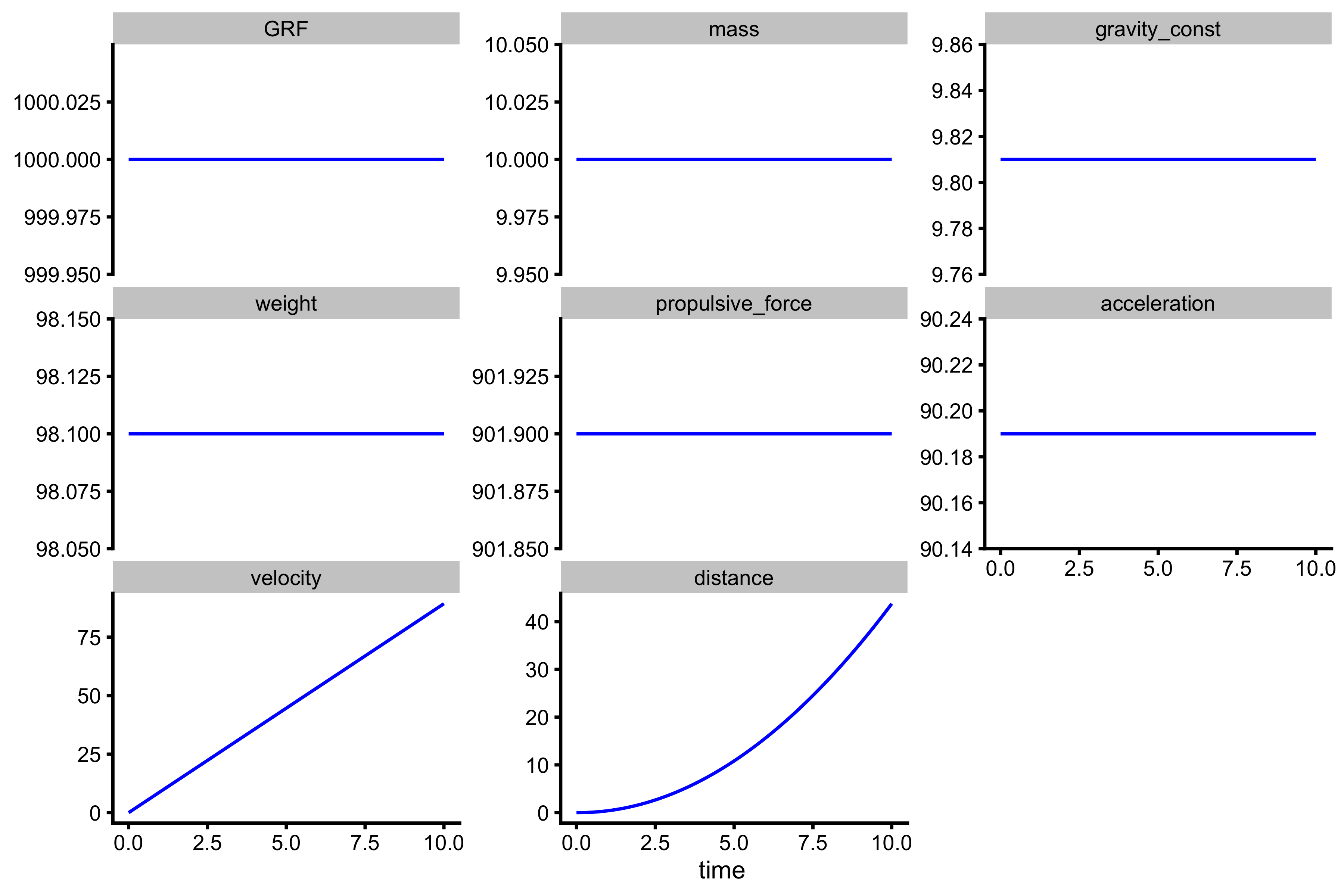
What we got is this weird curve. What is interesting to notice is that change in velocity is equal to area under curve of the acceleration (hence \(v = a \times t\)), and change in distance is equal to area under curve of the velocity. From the picture above, we see that the area under the velocity curve represents triangle, with the bottom side (\(a\)) equal to \(t\), and top side (\(b\)) equal to \(a \times t\). Since the area for the triangle is equal to \(\frac{a \times b}{2}\), then the equation for distance is equal to:
\[ d = d_0 + \frac{1}{2}at^2 \] This is, of course, true in the case when there is constant acceleration.
How is power (\(P\)) calculated? So, power is the ability to do work (\(W\)) in a unit of time (\(t\)). Work is defined as the force multiplied by distance:
\[ W = F \times d \]
So, power is thus:
\[ \begin{aligned} P &= \frac{W}{t} \\ P &= \frac{F\times d}{t} \\ \end{aligned} \]
Since \(\frac{d}{t}\) is equal to velocity \(v\), then the power is equal to:
\[ P = F \times v \]
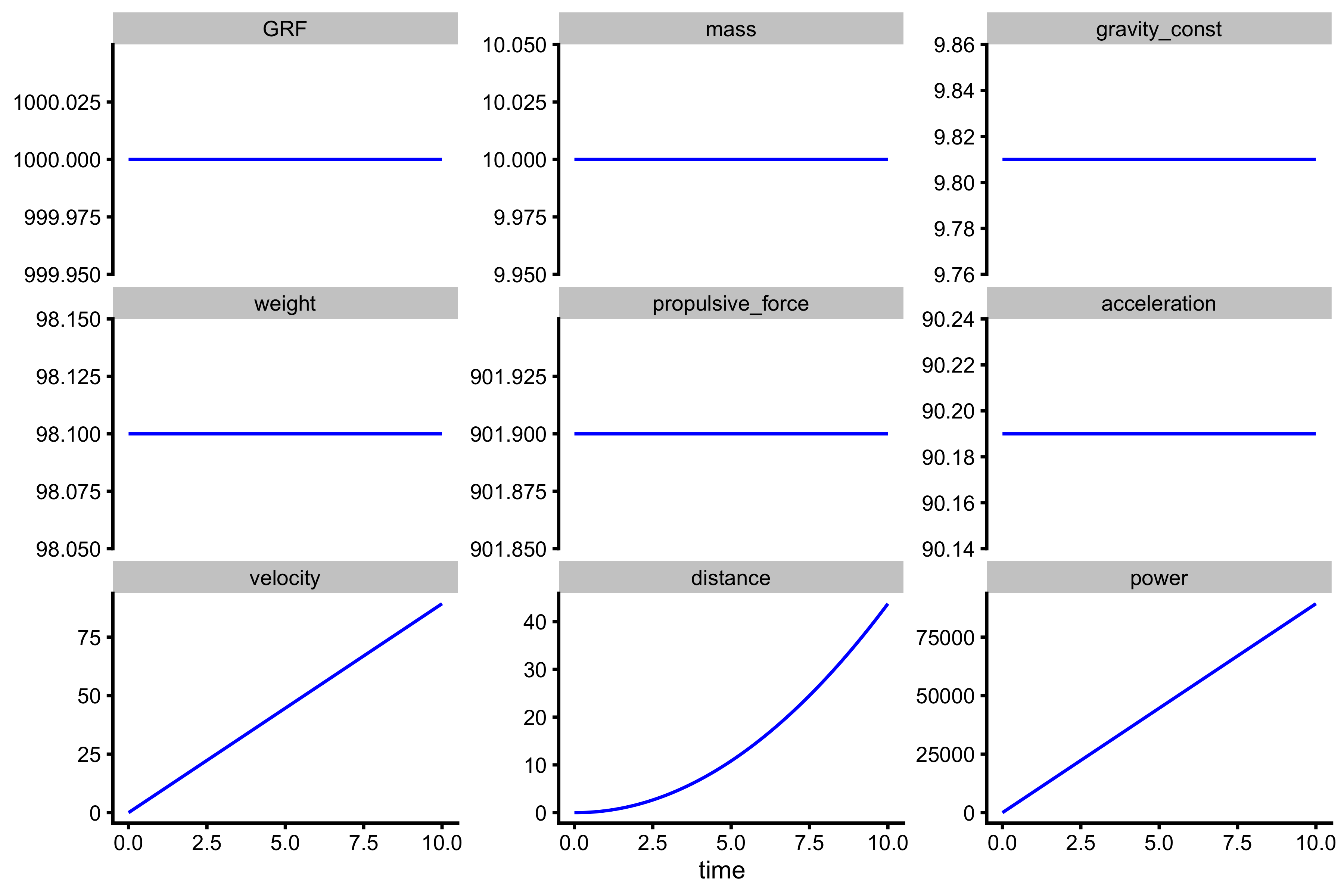
But which force should be used? GRF (total force) or propulsive force (net)? The work done by GRF, will be used to increase both potential energy (\(E=m\times g\times d\); assuming this motion is vertical, which it is) and kinetic energy (\(E=\frac{m\times v^2}{2}\)), while work done by net force will only be used to increase kinetic energy. Thus, to calculate the power, GRF should be used. We can plot that as well:
kinetics_data <- kinetics_data %>%
  mutate(power = GRF * velocity)

plot_data <- gather(kinetics_data, "variable", "value", -time) %>%
  mutate(variable = factor(variable, levels = c(
    "GRF",
    "mass",
    "gravity_const",
    "weight",
    "propulsive_force",
    "acceleration",
    "velocity",
    "distance",
    "power"
  )))

ggplot(plot_data, aes(x = time, y = value)) +
  theme_cowplot(8) +
  geom_line(color = "blue") +
  facet_wrap(~variable, scales = "free_y") +
  ylab(NULL)
Mean Velocity, Mean Force, Mean Power
Rather than juggling with all the data points depicted in the figures above, we want to aggregate them somehow. For example, we want to know the mean velocity over that 10second. We can simply calculate that as:
\[ \bar{v} = \frac{d}{t} \]
Or the distance \(d\) covered over time \(t\). Another way to do it, would be to represent velocity chat with a square or bar. So, the area under the velocity line, we can to represent with the bar that has an equal surface. So, using the velocity \(v_{peak}\) reached after time \(t\), and time \(t\) to calculate surface we get the following:
\[ \begin{aligned} Area_{triangle} &= Area_{square} \\ \frac{v_{peak} \times t}{2} &= \bar{v} \times t \\ \bar{v} = \frac{v_{peak}}{2} \end{aligned} \] From the above equation, mean velocity is equal to half of the peak velocity. Graphically that looks like this:
ggplot(kinetics_data, aes(x = time, y = velocity)) +
  theme_cowplot() +
  geom_line(color = "blue") +
  geom_hline(yintercept = max(kinetics_data$velocity) / 2, linetype = "dashed")
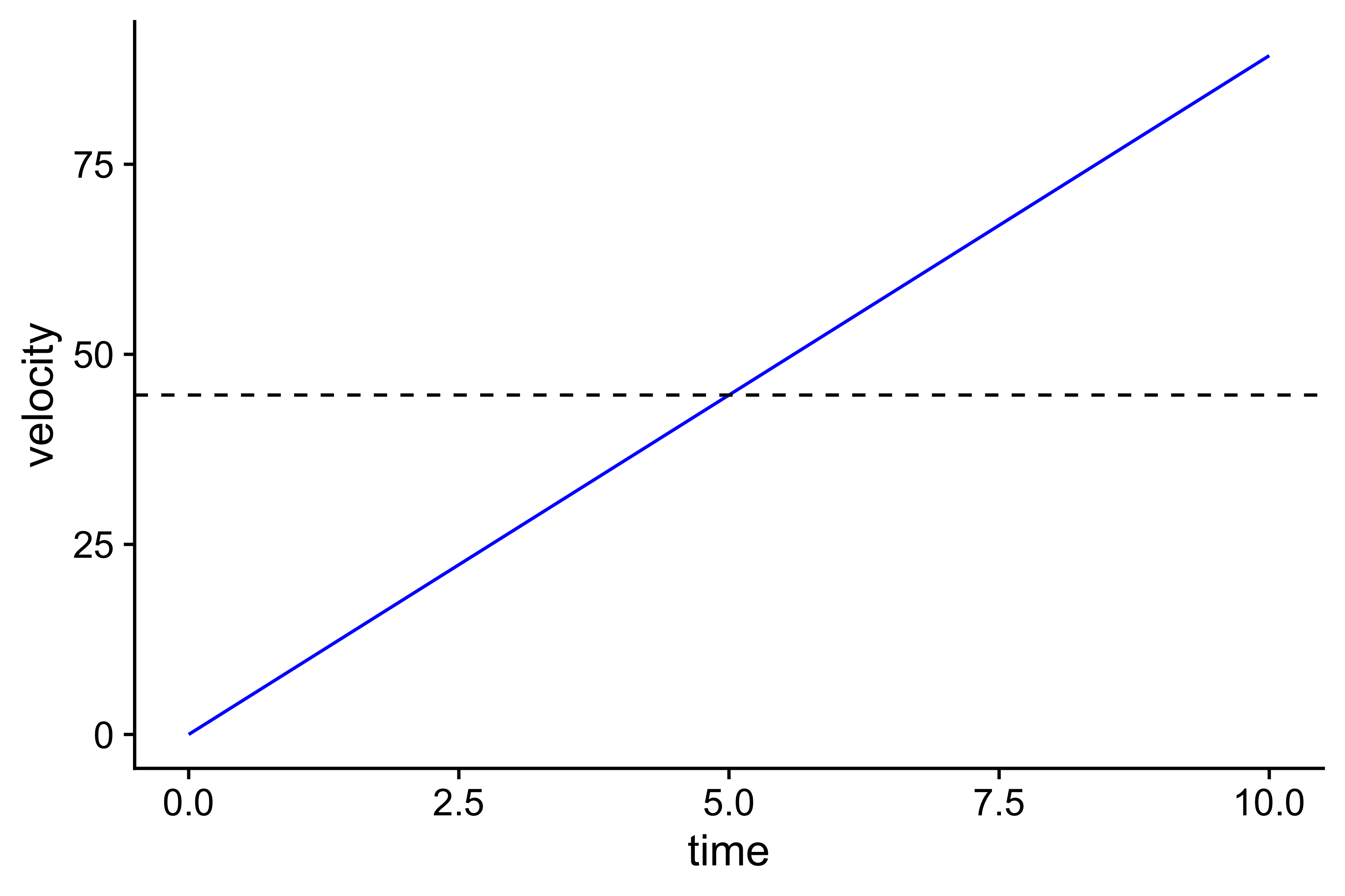
Please NOTE that this simple relationship between \(v_{peak}\) and \(\bar{v}\) (or \(v_{mean}\)) is only true when there is CONSTANT acceleration.
To calculate mean force (GRF) we can utilize two approaches. The first approach uses work done to increase potential and kinetic energy. Since work is equal to force multiplied by distance, we get the following:
\[ \begin{aligned} W &= \bar{F} \times d \\ E_{potential} + E_{kinetic} &= \bar{F} \times d \\ m \times g \times d \: + \frac{m\times v^2}{2} &= \bar{F} \times d \\ \bar{F} &= m \times g + \frac{m \times v^2}{2d} \end{aligned} \]
Other approach is using impulse (\(I\)) and momentum (\(M\)):
\[ \begin{aligned} I &= M \\ \bar{F_{net}} \times t &= m \times v \\ (\bar{F_{GRF}} - w) \times t &= m \times v \\ \bar{F_{GRF}} &= \frac{m\times v}{t} + w \end{aligned} \]
What is the difference between the two? If you calculate the mean force using these two approached for the above example, the results would be the same. It is thus easy to conclude that they are the same. But that is BLOODY WRONG. Once the force starts being non-constant, these two will differ. The first time when I wrote the simulator, I was getting different answers (i.e. different mean forces) using these two methods. I think I was breaking my head for more than a week, trying to figure out if my simulation code is wrong, or there is something that I don’t get.
The problem was in the term mean. What does “mean mean”? It is the average of some value OVER some other. Let’s take velocity from our example. We have plotted it AGAINST time, but let’s see what happens when we plot it against distance (or position):
ggplot(kinetics_data, aes(x = distance, y = velocity)) +
  theme_cowplot() +
  geom_line(color = "blue")
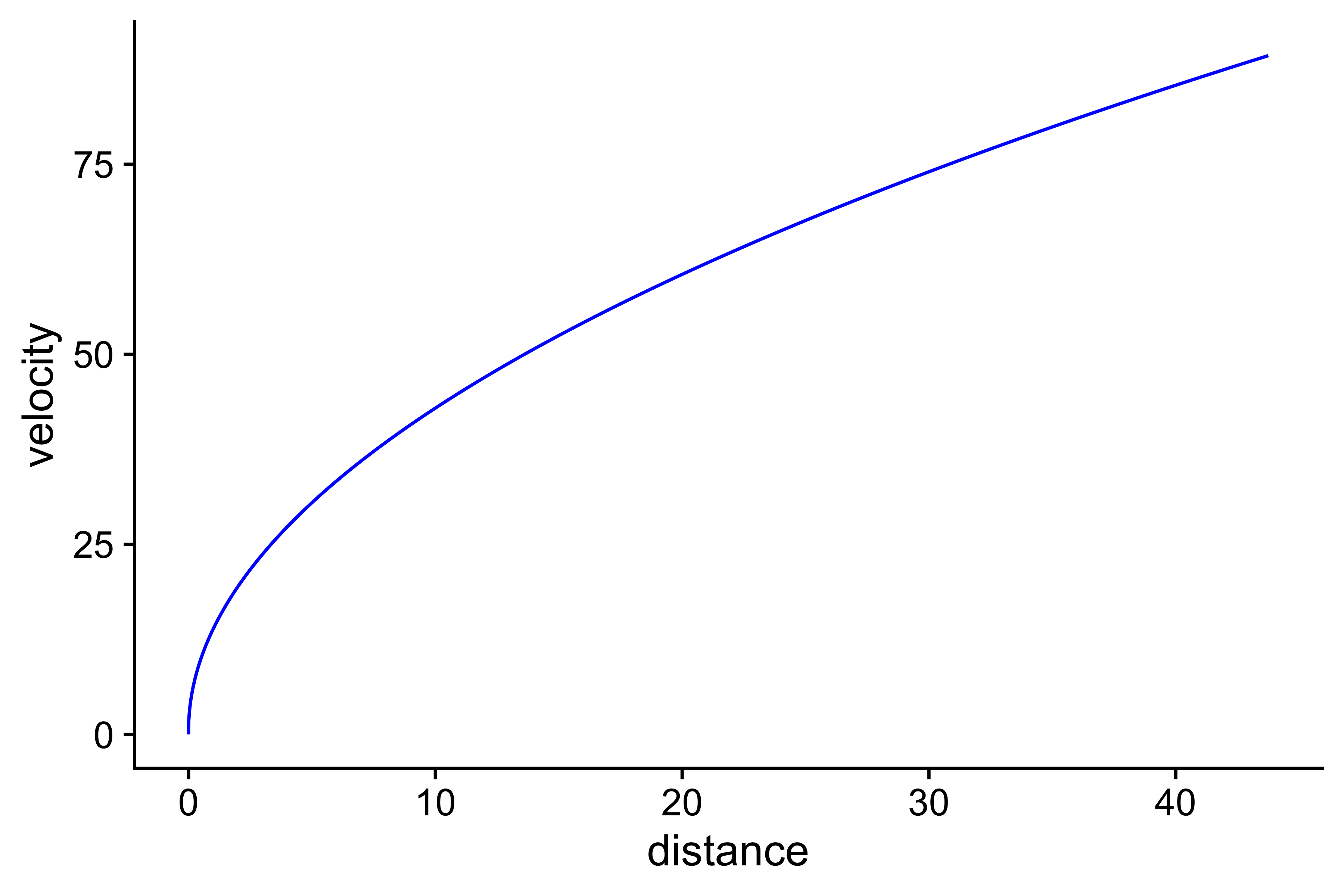
Luckily, mean velocity OVER time is equal to mean velocity OVER distance (since velocity is the first derivative of distance). But this is not the case for force. Thus there are two mean forces: one mean force OVER time, and second, mean force OVER distance. They are the same when the force is constant, but different when the force fluctuates. If we use work to calculate mean force, we will get mean force over a distance. If we use impulse and momentum to calculate mean force, we will get mean force over time. This distinction is often forgotten, and these two means are used interchangeably erroneously. This often the case in some optimization models, but we will discuss these issues later in other vignettes.
To make distinction, in vjsim I am using two mean forces: mean_GRF_over_time and mean_GRF_over_distance.
How is the mean power calculated? It is simple work done divided by total time. As already stated, work done by the force is used to increase kinetic and potential energy. Thus, the mean power is equal to:
\[ \begin{aligned} \bar{P} &= \frac{W}{t} \\ \bar{P} &= \frac{E_{potential} + E_{kinetic}}{t} \\ \bar{P} &= \frac{m \times g \times d \: + \frac{m\times v^2}{2}}{t} \\ \end{aligned} \]
It is important to keep in mind that we differ between instantaneous values of velocity, distance, forces, power as well as summaries (usually means and peaks) over a certain time period or distance. In the vertical jump example, we have limited push-off distance; thus we are interested in means and peaks over push-off distance.
But wait, Force Generator doesn’t produce constant force?!?
The “problem” with our Force Generator is that it produces force that depends on the position on push-off distance (due to Force-Length characteristic; based on decline_rate and peak_location parameters), velocity (due to Force-Velocity characteristic; based on max_force and max_velocity parameters), and time (due to Force-Time characteristic; based on time_to_max_activation parameter). This means that current acceleration depends on the current Force Generator force output, that depends on current velocity, current position, and current time:
\[ a = \frac{F_{gen}(position, velocity, time) - w}{m} \]
This means that we need to take small time steps as we did in the code above, and iteratively calculate acceleration, velocity, and distance. This method is called Euler’s method. So at current instant in time (\(t\)), we assume linear relationships and calculate next (\(t+1\)) velocity, and position using small changes in time (\(dt\), or time_step):
\[ \begin{aligned} acceleration_{t} &= \frac{F_{gen}(position_{t}, velocity_{t}, time_{t}, parameters) - w}{m} \\ velocity_{t+1} &= velocity_{t} + acceleration_{t} \times dt \\ distance_{t+1} &= distance_{t} + velocity_{t} \times dt \end{aligned} \]
This Force Generator output is generated by vjsim::fgen_get_output discussed in the previous vignette.
The method implemented in vjsim is slightly more complicated version of the simple Euler method, called Runge-Kutta and involves some middles steps (for example, in the above equation, you can improve precision of the distance calculation by assuming constant acceleration between \(v_{t}\) and \(v_{t+1}\) and thus use \(distance_{t} + velocity_{t} \times dt + \frac{acceleration_{t} \times dt^2}{2}\)). Time step used in vjsim is 0.001s. Selecting a time step involves the trade-off between speed of execution and precision. But 0.001s seems like a good value for our purposes of simulating vertical jump and also probing the system sensitivity (discussed later).
Jump trace in vjsim
Let’s do the jump in vjsim using the following parameters (see code below) and function vjsim::vj_simulate:
vertical_jump <- vjsim::vj_simulate(
  mass = 85,
  weight = 85 * 9.81,
  push_off_distance = 0.4,
  gravity_const = 9.81,
  time_step = 0.001,

  # Parameters of the Force Generator
  max_force = 3000,
  max_velocity = 4,
  decline_rate = 1.05,
  peak_location = -0.06,
  time_to_max_activation = 0.3
)
vjsim:vj_simulate returns a list object with two elements: summary and trace. Let’s first explore trace. Here is the full table:
datatable(vertical_jump$trace, rownames = FALSE) %>%
  formatRound(columns = 1:ncol(vertical_jump$trace), digits = 3)
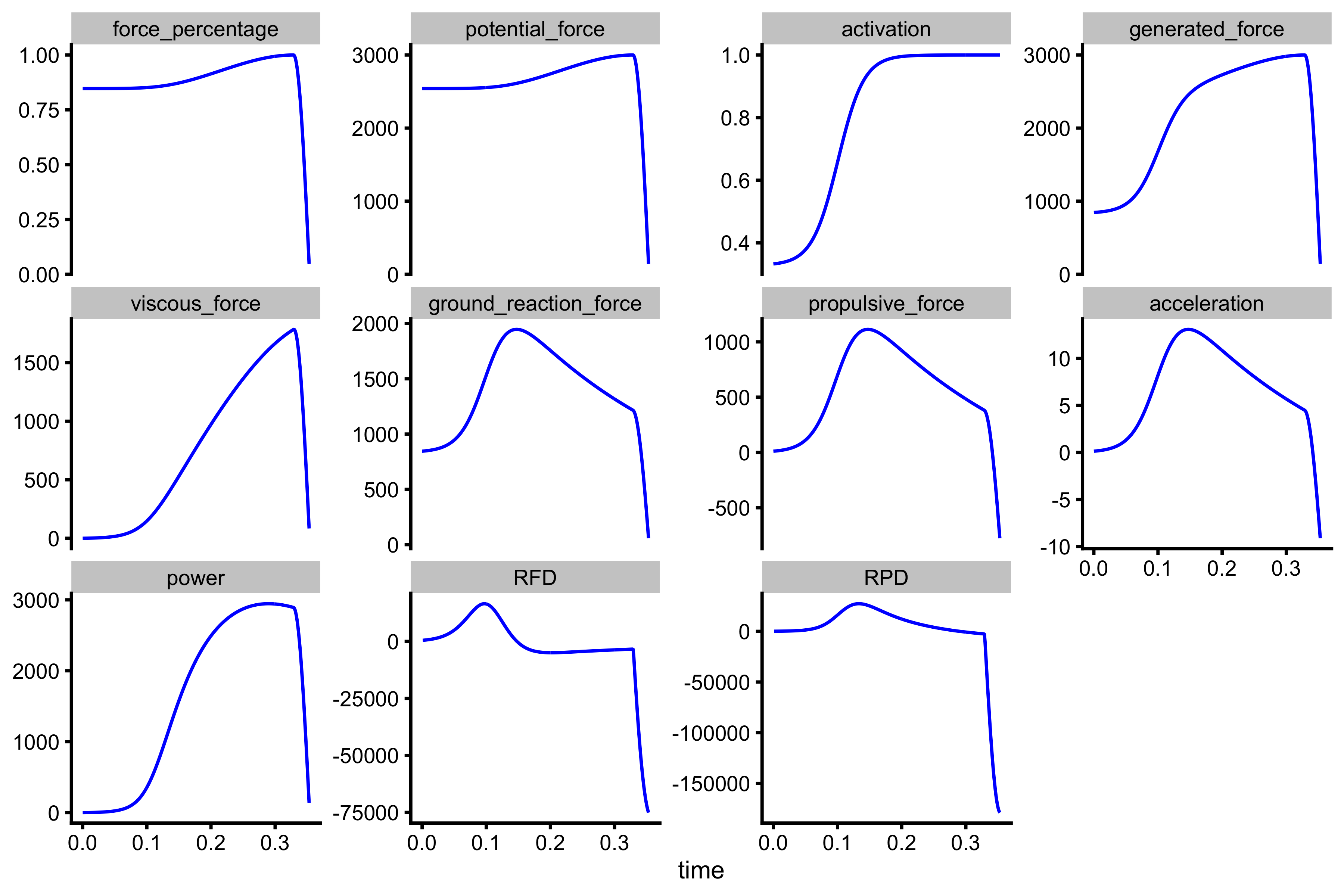
Plotting this is a much better way to see the vertical jump simulation results. Let’s plot against time.
plot_data <- gather(vertical_jump$trace, "variable", "value", -(1:15)) %>%
  mutate(variable = factor(
    variable,
    levels = c(
      "force_percentage",
      "potential_force",
      "activation",
      "generated_force",
      "viscous_force",
      "ground_reaction_force",
      "propulsive_force",
      "acceleration",
      "power",
      "RFD",
      "RPD"
    )
  ))

ggplot(plot_data, aes(x = time, y = value)) +
  theme_cowplot(8) +
  geom_line(color = "blue") +
  facet_wrap(~variable, scales = "free_y") +
  ylab(NULL)
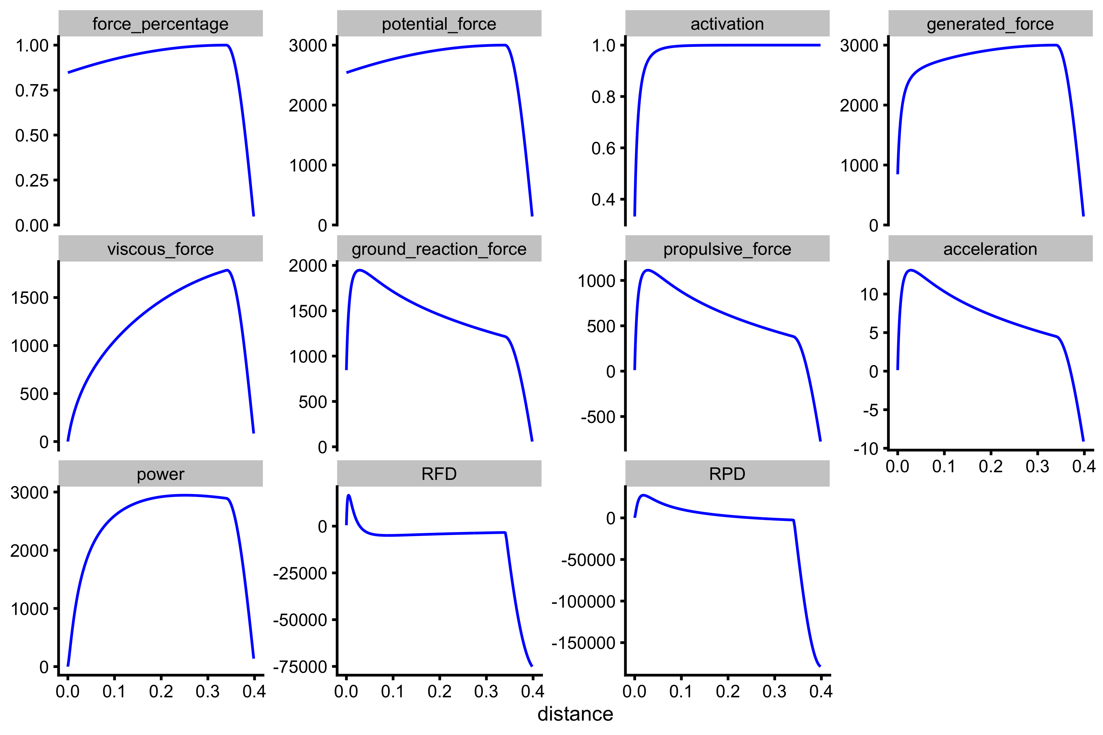
Or we can plot against distance:
ggplot(plot_data, aes(x = distance, y = value)) +
  theme_cowplot(8) +
  geom_line(color = "blue") +
  facet_wrap(~variable, scales = "free_y") +
  ylab(NULL)
RFD and RPD are additional variables produces by vjsim::vj_simulate and represent rate-of-force-development (GRF to be more precise) and rate-of-power-development. It represents a change in GRF and power divided by the time step (i.e. 0.001). mean_RFD and mean_RPD are calculated by dividing their peak values by the time it takes to reach the peak.
The summary list represents, well, the summary of the jump. We can also call these performance metrics.
df <- as.data.frame(t(vertical_jump$summary))
colnames(df)[1] <- "value"
round(df, 2)
#>                                         value
#> mass                                    85.00
#> weight                                 833.85
#> push_off_distance                        0.40
#> gravity_const                            9.81
#> take_off_distance                        0.40
#> take_off_time                            0.35
#> take_off_ground_reaction_force          57.80
#> take_off_propulsive_force             -776.05
#> take_off_velocity                        2.37
#> height                                   0.29
#> mean_GRF_over_distance                1431.47
#> mean_GRF_over_time                    1403.63
#> mean_velocity                            1.13
#> work_done                              570.01
#> impulse                                201.13
#> mean_power                            1614.75
#> mean_RFD                             13244.60
#> mean_RPD                             10156.44
#> peak_GRF                              1946.96
#> peak_GRF_time                            0.15
#> peak_GRF_distance                        0.03
#> peak_velocity                            2.42
#> peak_velocity_time                       0.34
#> peak_velocity_distance                   0.37
#> peak_power                            2945.37
#> peak_power_distance                      0.25
#> peak_power_time                          0.29
#> peak_RFD                             16527.99
#> peak_RFD_distance                        0.00
#> peak_RFD_time                            0.10
#> GRF_at_100ms                          1515.78
#> GRF_at_200ms                          1760.75
#> peak_RPD                             27244.40
#> peak_RPD_distance                        0.02
#> peak_RPD_time                            0.13
#> diff_peak_to_take_off_velocity           0.05
#> ratio_peak_to_take_off_velocity          1.02
#> diff_mean_to_take_off_velocity          -1.24
#> ratio_mean_to_take_off_velocity          0.48
#> diff_mean_to_peak_velocity              -1.29
#> ratio_mean_to_peak_velocity              0.47
#> diff_mean_to_peak_power              -1330.62
#> ratio_mean_to_peak_power                 0.55
#> diff_mean_GRF_over_distance_to_time     27.83
#> ratio_mean_GRF_over_distance_to_time     1.02
#> mean_velocity_as_TOV_half                1.18
This table gives a summary of the vertical jump performance. It includes constraints of the system (mass, weight, push-off distance, gravity constant), latest values at the take_off (take-off time, take-off distance, take-off velocity, take-off GRF, and take-off propulsive force), height of the jump (calculated using ballistic equation and take-off velocity), as well mean and peak summaries for velocity, force, power, RFD, and RPD. Peak summaries also include the location (time and distance) of the peak occurrence.
Please note the difference between mean_GRF_over_distance (1431.47N) and mean_GRF_over_time (1403.63N). You can compare the GRF traces in the above figures when plotting against time or distance. Another thing to notice is the ratio between peak_velocity (2.42\(ms^-1\)) and mean_velocity (1.13\(ms^-1\)) which is equal to 2.14, while it should be equal to 2 if there is constant acceleration. Also note that the peak_velocity (2.42\(ms^-1\)) differs from take_off_velocity (2.37\(ms^-1\)).
Before continuing with reading, I highly suggest either playing with the code or using the Shiny App (this will take you to the shinyapps.io) by click on the previous link or by running the following code:
vjsim::run_simulator()
This will give you some feel for the vertical jump simulator and how changing Force Generator parameters affect jump kinematics and kinetics.
Probing vertical jump performance sensitivity to parameter changes
Now that we have some glimpse into how the simulator works, we might be interested in how the change in Force Generator parameters affect jump performance (i.e. height, mean velocity, peak power or any other performance metric) and which Force Generator parameter change yields the biggest change in the performance metric of interest. In other words, answering which Force Generator parameter is the most important.
To do so, we need to probe the simulator in order to estimate sensitivity of the performance metric of interest. There is one problem though - the Force Generator parameters are not on the same scale. Thus, we need to normalize or standardize parameter change using the multiplication. For example, we want to check how does change of 10% (i.e. multiplied by 1.1) in a given parameter affect the performance metric of interest (i.e height), as well how does the change of -10% (i.e. multiplied by 0.9) affect the performance metric. In plain English, I want to answer the following question “If I increase max force for 10%, will I get more improvement in jump height compared if I increase max velocity for 10%”. Here is how to do it in vjsim:
probing_data <- vjsim::probe_vj(
  mass = 85,
  change_ratio = c(0.9, 1, 1.1),
  aggregate = "raw",
  # Parameters forwarded to vj_sim
  weight = 85 * 9.81,
  push_off_distance = 0.4,
  gravity_const = 9.81,
  time_step = 0.001,
  # Parameters of the Force Generator
  max_force = 3000,
  max_velocity = 4,
  decline_rate = 1.05,
  peak_location = -0.06,
  time_to_max_activation = 0.3
)

datatable(probing_data, rownames = FALSE) %>%
  formatRound(columns = 1:ncol(probing_data), digits = 2)
How does this work? First, we need to have initial Force Generator parameter values. Then we take and change one parameter and modify it using change_ratio (i.e. multiply by 0.9, 1, and 1.1), while keeping all the other parameters the same (i.e. using initial values). Then we repeat this for all Force Generator parameters.
As you will notice from the table, its not all Forge Generator parameters that are probed. The only exception are the decline rate and peak location, since they are assumed not to be changeable. Thus, we probe the changes in mass (i.e. losing some bodyweight), push-off distance (i.e. taking deeper or shallower squat position), max force (i.e. getting stronger), max velocity (i.e. getting faster), and time to max activation (i.e. getting more explosive).
The sensitivity is hard to be grasped from the table, so let’s plot these. But before, we need to invert the change for the mass and time to max activation, because improving these means decreasing them. This puts them in line with other parameters, where improving implies increasing. We are also going to remove certain performance metrics that are of no interest at this stage.
# Invert for mass and time_to_max_activation
probing_data$change_ratio <- ifelse(
  probing_data$probing == "time_to_max_activation",
  1 / probing_data$change_ratio,
  probing_data$change_ratio
)

probing_data$change_ratio <- ifelse(
  probing_data$probing == "mass",
  1 / probing_data$change_ratio,
  probing_data$change_ratio
)


plot_data <- gather(probing_data, key = "variable", value = "value", -(1:13)) %>%
  filter(variable %in% c(
    "height",
    "take_off_time",
    "mean_velocity",
    "peak_velocity",
    "take_off_velocity",
    "mean_GRF_over_distance",
    "mean_GRF_over_time",
    "peak_GRF",
    "peak_power",
    "mean_power",
    "peak_RFD",
    "peak_RPD"
  ))

plot_data$reverse <- plot_data$probing %in% c("mass", "time_to_max_activation")

gg <- ggplot(plot_data, aes(x = change_ratio, y = value, color = probing, linetype = reverse)) +
  theme_cowplot(6) +
  geom_line() +
  facet_wrap(~variable, scales = "free_y") +
  xlab("Normalized parameter change") +
  ylab(NULL) +
  scale_color_manual(values = c(
    "mass" = "#4D4D4D",
    "max_force" = "#5DA5DA",
    "max_velocity" =  "#FAA43A",
    "push_off_distance" = "#60BD68",
    "time_to_max_activation" = "#B276B2"
  ))
gg
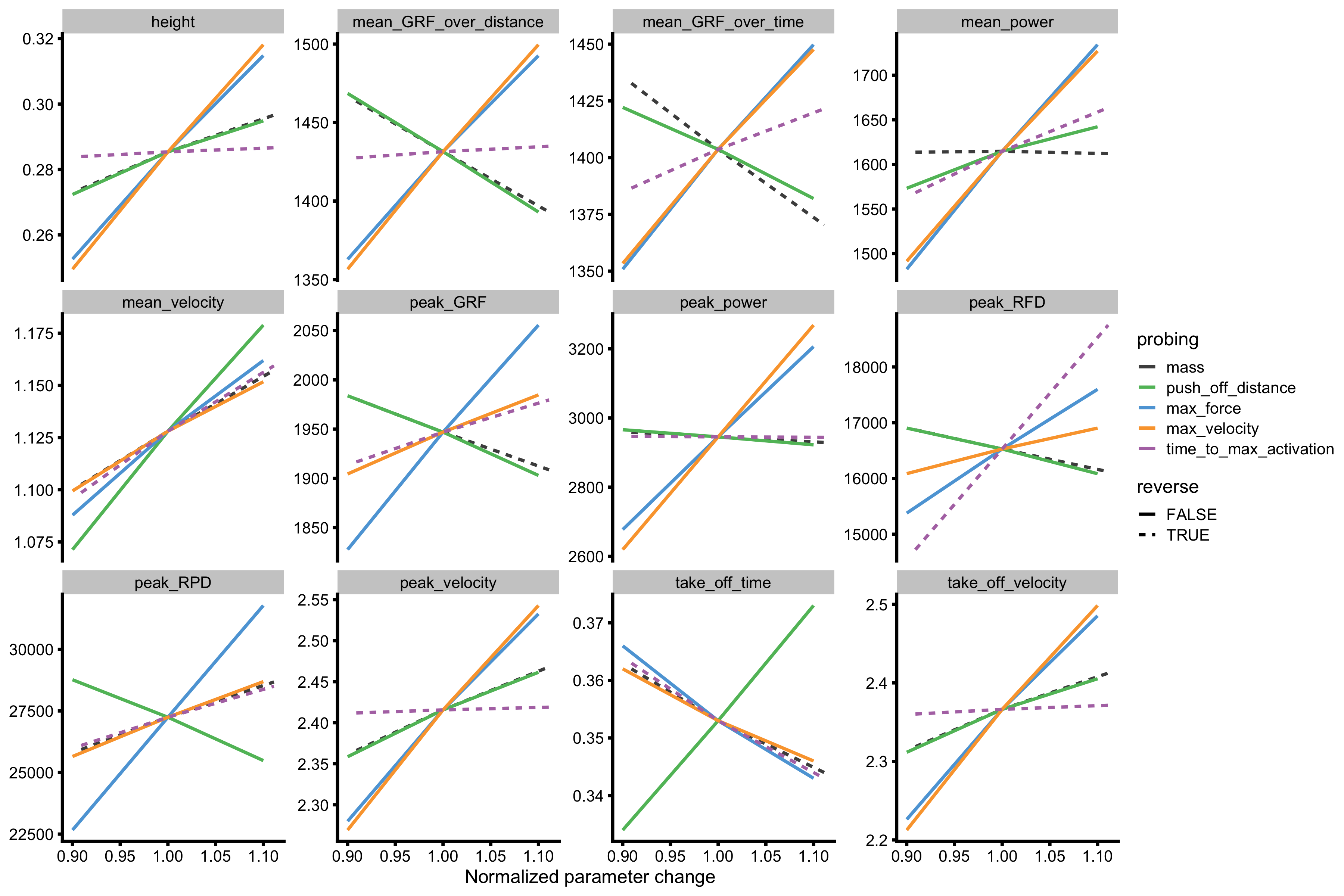
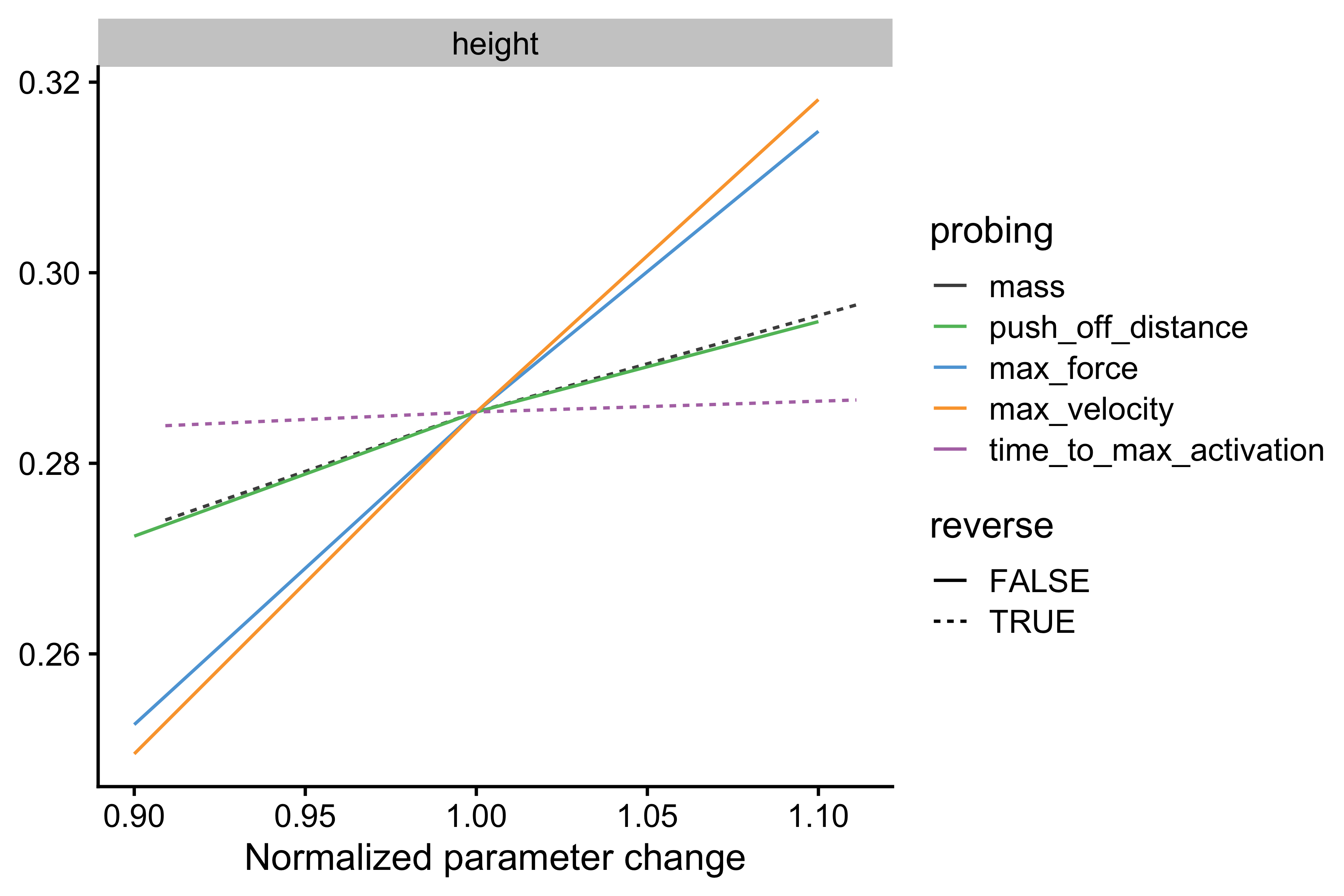
For example, if we take only jump height (see below for better zoom), given the initial Forge Generator parameters, it seems that increasing max velocity (for 10%) will yield slightly larger improvements than increasing max force. This doesn’t tell us anything regarding which Force Generator parameter change is easier to create - for example, 10% improvement in max velocity can be very hard to do, compared to 20% improvement in max force. The simulator doesn’t know this - it is up to us, coaches or anyone with subject-matter knowledge, to interpret these for the potential intervention. And besides, keep in mind that this is only a model, it thus represent the sand box or the Small World.
gg <- ggplot(
  filter(plot_data, variable == "height"),
  aes(x = change_ratio, y = value, color = probing, linetype = reverse)
) +
  theme_cowplot(12) +
  geom_line() +
  facet_wrap(~variable, scales = "free_y") +
  xlab("Normalized parameter change") +
  ylab(NULL) +
  scale_color_manual(values = c(
    "mass" = "#4D4D4D",
    "max_force" = "#5DA5DA",
    "max_velocity" =  "#FAA43A",
    "push_off_distance" = "#60BD68",
    "time_to_max_activation" = "#B276B2"
  ))
gg
Similar question that can be asked is “If I change a particular Force Generator parameter, in which performance metric I can expect the biggest change”. Here we have another problem - the performance metrics are not on the same scale (i.e. height vs. mean power), so we need to normalize or standardize the change of the performance metric. We do so by using aggregate = "ratio" parameter in vjsim::probe_vj. This will divide the changed performance metric with the initial performance metric.
Our initial value for max force is 3,000N. Now we are interested which performance metric changes the most when max force changes.
# Need this package to label the lines
# install.packages("directlabels")
require(directlabels)


probing_data <- vjsim::probe_vj(
  mass = 85,
  change_ratio = c(0.9, 0.95, 1, 1.05, 1.1),
  aggregate = "ratio",
  # Parameters forwarded to vj_sim
  weight = 85 * 9.81,
  push_off_distance = 0.4,
  gravity_const = 9.81,
  time_step = 0.001,
  # Parameters of the Force Generator
  max_force = 3000,
  max_velocity = 4,
  decline_rate = 1.05,
  peak_location = -0.06,
  time_to_max_activation = 0.3
)

plot_data <- gather(probing_data, key = "variable", value = "value", -(1:13)) %>%
  filter(
    variable %in% c(
      "height",
      "take_off_time",
      "mean_velocity",
      "peak_velocity",
      "take_off_velocity",
      "mean_GRF_over_distance",
      "mean_GRF_over_time",
      "peak_GRF",
      "peak_power",
      "mean_power",
      "peak_RFD",
      "peak_RPD"
    )
  )

gg <- ggplot(
  filter(plot_data, probing == "max_force"),
  aes(x = change_ratio, y = value, color = variable)
) +
  theme_cowplot(12) +
  geom_line() +
  facet_wrap(~probing, scales = "free_y") +
  xlab("Normalized parameter change") +
  ylab(NULL) +
  xlim(c(0.9, 1.2))
direct.label(gg, list("last.bumpup", cex = 0.7))
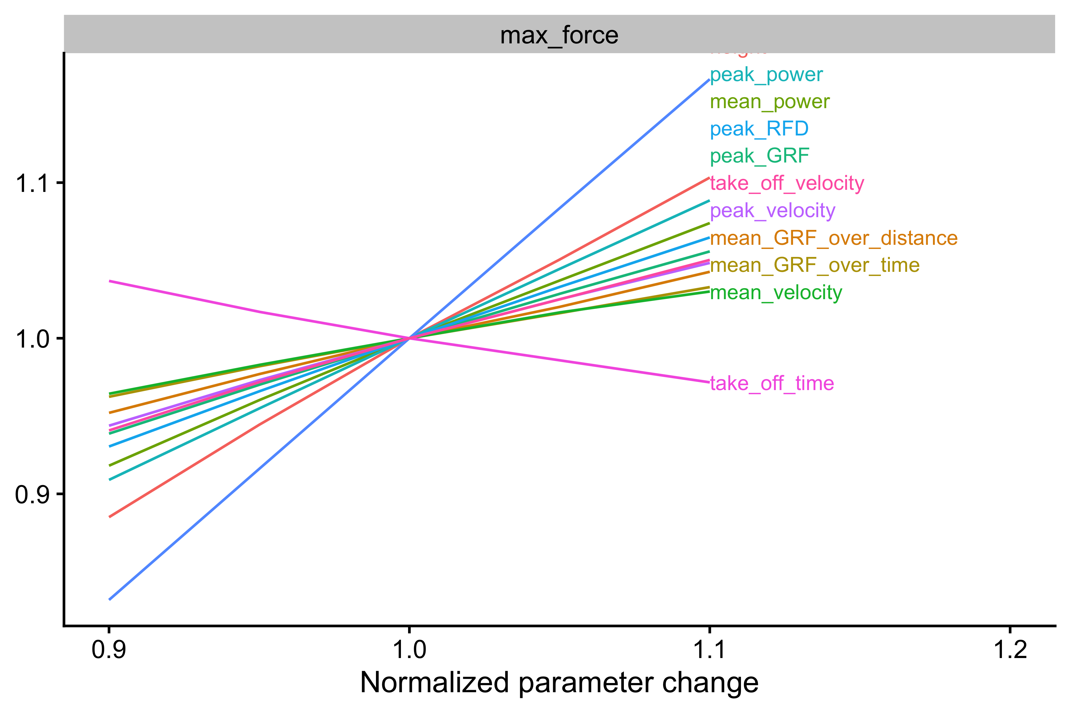
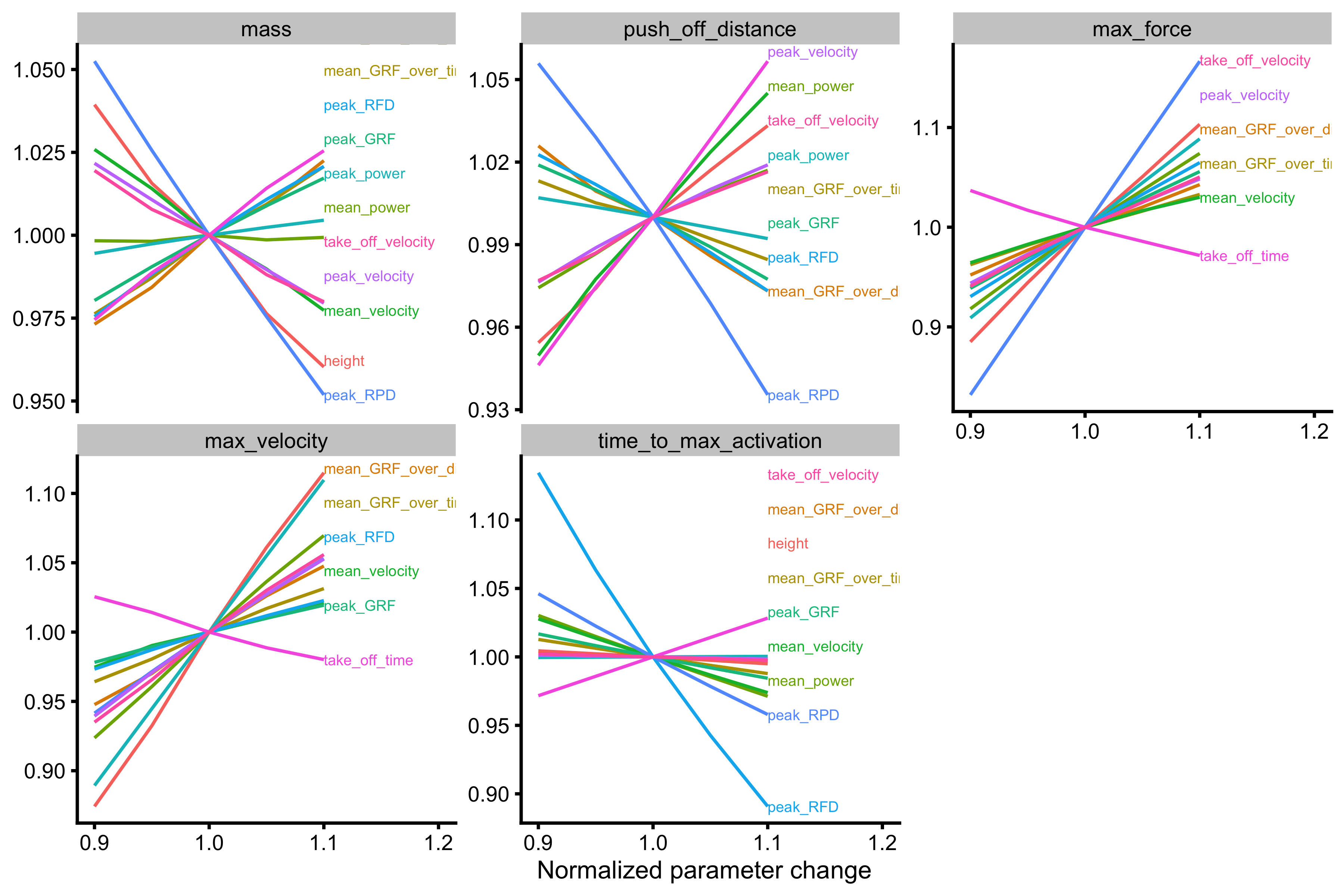
As can be seen from the figure above, it seems that the change in max force will have the biggest impact on peak_RPD, followed by jump height. We can do this for other Force Parameters:
gg <- ggplot(
  plot_data,
  aes(x = change_ratio, y = value, color = variable)
) +
  theme_cowplot(8) +
  geom_line() +
  facet_wrap(~probing, scales = "free_y") +
  xlab("Normalized parameter change") +
  ylab(NULL) +
  xlim(c(0.9, 1.2))
direct.label(gg, list("last.bumpup", cex = 0.4))
Shiny App
Now start playing with the code or with the Shiny App by click on the previous link or by running the following code:
vjsim::run_simulator()
The Shiny App will allow you much more interactive environment for exploring the vjsim.