Squat jump testing dataset
# Install vjsim if you haven't already by running the following commands
# install.packages("devtools")
# devtools::install_github("mladenjovanovic/vjsim")

# Install bmbstats if you haven't already by running the following commands
# devtools::install_github("mladenjovanovic/bmbstats")

# Install tidyverse and cowplot packages
# install.packages(c("tidyverse", "cowplot", "DT", "boot"), dependencies = TRUE)

library(vjsim)
library(tidyverse)
library(cowplot)
library(DT)
library(boot)
library(bmbstats)
Before reading this vignette, please read Introduction to vjsim, Simulation in vjsim, Profiling in vjsim, Optimization in vjsim and Exploring vjsim vignettes by running:
vignette("introduction-vjsim")
vignette("simulation-vjsim")
vignette("profiling-vjsim")
vignette("optimization-vjsim")
vignette("exploring-vjsim")
In this vignette I will demonstrate modeling features of the vjsim by using built in dataset testing_data. testing_data consists of N=5 individuals tested in the progressively loaded squat jump using jump mat. Jump mat provide aerial time that we need to convert to jump height. All but one athlete (“Chris”) has known push-off distance (that was measure before testing). Here is the dataset:
data("testing_data")

datatable(testing_data, rownames = FALSE) %>%
  formatRound(columns = 1:ncol(testing_data), digits = 2)
To convert aerial time to jump height we will use vjsim::get_height_from_aerial_time function, which uses simple ballistic equation:
\[ h = \frac{1}{8}\times g \times t_{aerial}^2 \]
Here is the code:
testing_data <- testing_data %>%
  mutate(height = vjsim::get_height_from_aerial_time(aerial_time))
We can plot the data:
ggplot(testing_data, aes(x = external_load, y = height)) +
  theme_cowplot(8) +
  geom_smooth(method = "lm") +
  geom_point() +
  facet_wrap(~athlete, scales = "free")

The gray band around the line represents the confidence band (or let’s call it uncertainty band; some call is compatibility band or interval) around the line. This is something we estimated as well using the bootstrap method in the previous vignettes. This confidence band for the line is used to make inferences to population, or to which true lines our data is compatible with (with 95% confidence)1. Since we have N=1 analysis, thus each athlete represents population, this uncertainty band can be seen as a compatibility band with individual’s true profile. This uncertainty can arise due too small number of observations, non-linear relationship between observations (which we are trying to model with a straight line), and measurement error (I will get back to this).
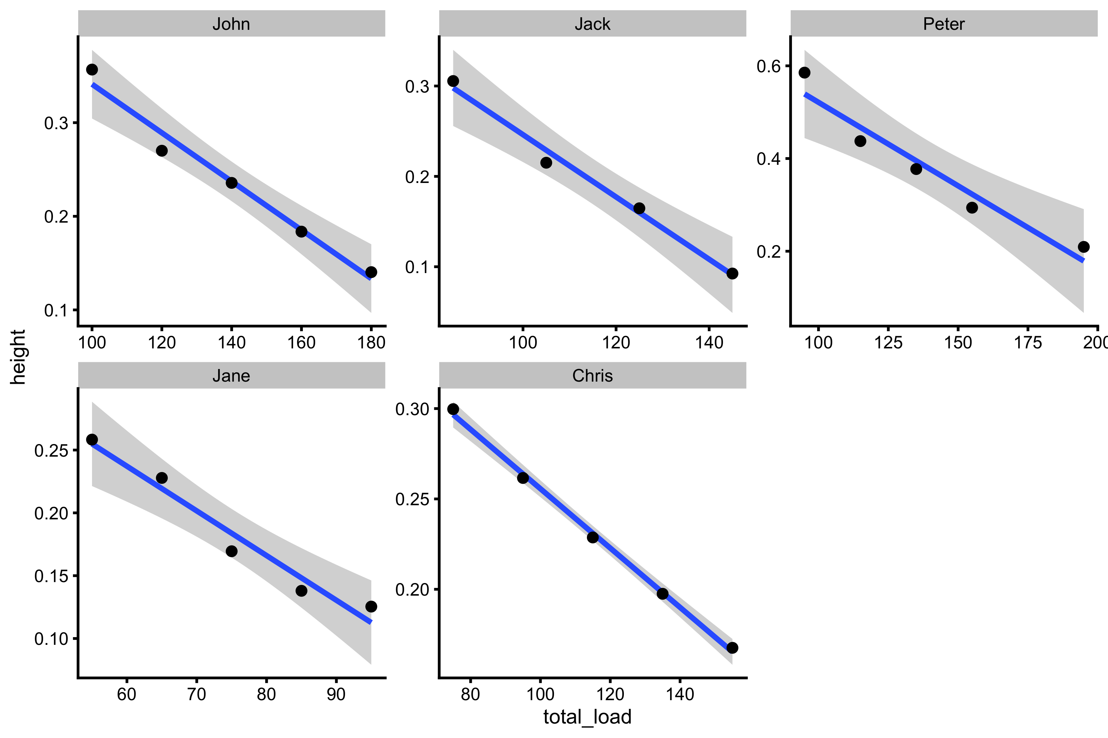
We can also plot total load, rater than external load:
testing_data <- testing_data %>%
  mutate(total_load = bodyweight + external_load)

ggplot(testing_data, aes(x = total_load, y = height)) +
  theme_cowplot(8) +
  geom_smooth(method = "lm") +
  geom_point() +
  facet_wrap(~athlete, scales = "free")
Modeling using Samozino method
This data represents the data that can be easily gathered in the field without the need for laboratory equipment (e.g., force plates; although these are now more common that before, as well as more affordable). One only needs jump mat, which is a simple contact mat that measures flight time. If we know someone’s push-off distance (which is measured and explained in (Samozino et al. 2010, 2008; Samozino 2018)), we can estimate mean force \(\bar{F}\) (mean ground reaction force; \(\bar{GRF}\)) over distance, and we can approximate mean velocity \(\bar{v}\) to be \(\frac{1}{2}\) of take-off velocity (TOV) (which is calculated from jump height or flight time). From this we can also calculate mean power \(\bar{P}\) during the push-off. This method is not exact, but as demonstrated in the previous vignettes and papers cited, it is good enough to be useful. For example, model doesn’t need to be factually 100% correct to be useful in practice (i.e., just remember the geocentric model vs heliocentric model). In my humble opinion, I would prefer for the Samozino model to show GRF~TOV graph rather than estimated mean velocity, particularly if the objective is to find the optimized intervention for improving vertical jump height. Thus, I would prefer to call it “mean force - take-off” velocity profile.
Here is how we can estimate mean force, mean velocity, TOV, and mean power using vjsim::get_samozino_jump_metrics function that takes load (i.e., bodyweight plus external load), push-off distance, and height as parameters. Since we are dealing with multiple individuals, I had to make a wrapper for this function to be used in the tidyverse framework:
jump_metric <- function(data) {
  samozino_metrics <- get_samozino_jump_metrics(
    mass = data$bodyweight + data$external_load,
    push_off_distance = data$push_off_distance,
    height = data$height
  )

  return(as.data.frame(samozino_metrics))
}

testing_data <- testing_data %>%
  # Need to add bodyweight so it is kept in the output
  group_by(athlete, bodyweight) %>%
  do(jump_metric(.))

datatable(testing_data, rownames = FALSE) %>%
  formatRound(columns = 1:ncol(testing_data), digits = 2)
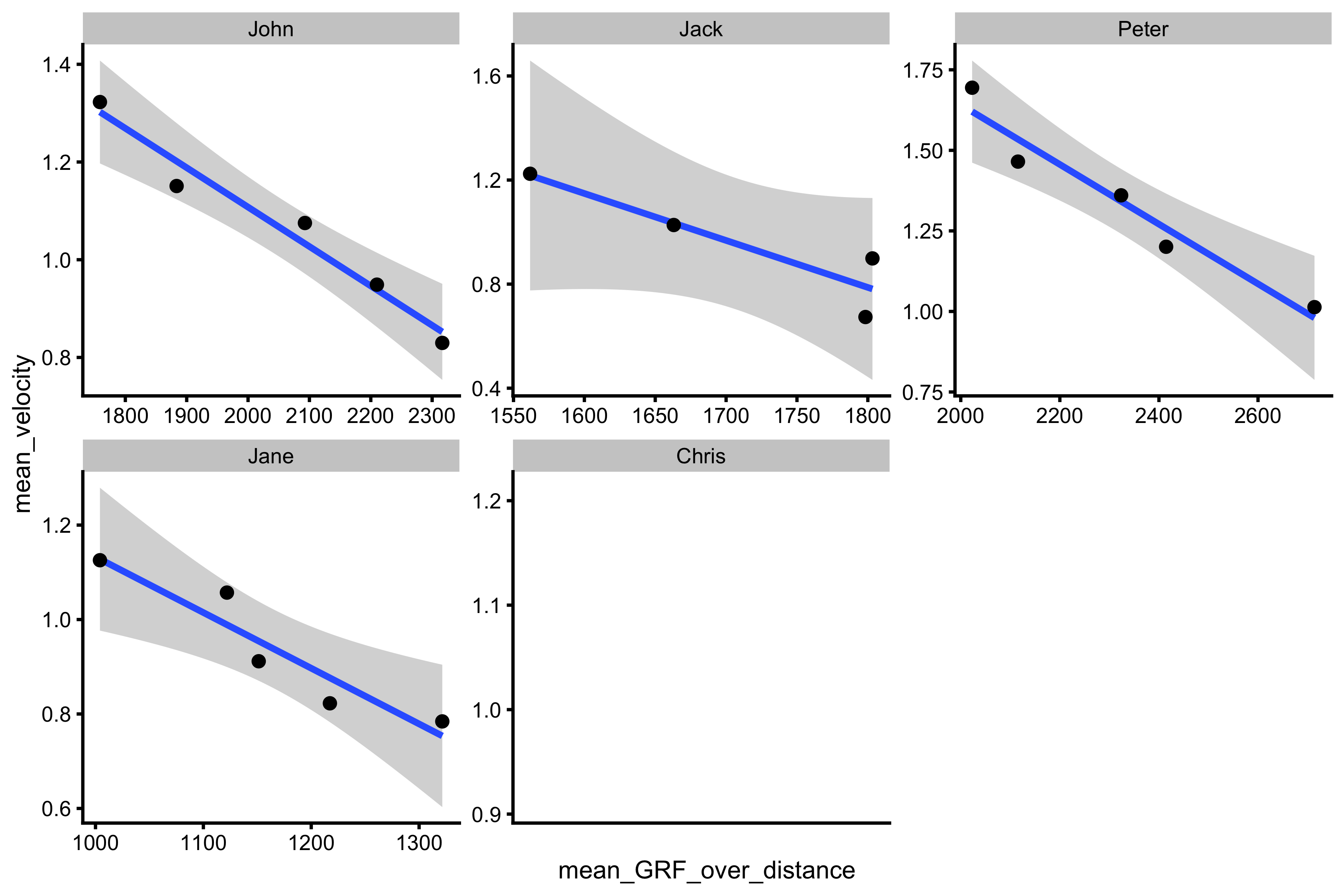
As can be seen, these could not be computed for Chris, since Chris lacks push-off distance data. Now we can plot both mean GRF - mean velocity profiles (or TOV, which I would personally prefer since there is no assumptions of uniform acceleration):
ggplot(testing_data, aes(x = mean_GRF_over_distance, y = mean_velocity)) +
  theme_cowplot(8) +
  geom_smooth(method = "lm") +
  geom_point() +
  facet_wrap(~athlete, scales = "free")
So now we have a profile. Using Samozino model, we can provide optimization estimates (discussed in the optimization vignette). This is done using vjsim::get_samozino_profile function. Here is an example for John:
john_data <- filter(testing_data, athlete == "John")

john_samozino_profile <- vjsim::get_samozino_profile(
  bodyweight = john_data$bodyweight,
  push_off_distance = john_data$push_off_distance,
  mean_GRF_over_distance = john_data$mean_GRF_over_distance,
  mean_velocity = john_data$mean_velocity
)

john_samozino_profile
#> $F0
#> [1] 3373.219
#>
#> $F0_rel
#> [1] 33.73219
#>
#> $V0
#> [1] 2.720893
#>
#> $Pmax
#> [1] 2294.542
#>
#> $Pmax_rel
#> [1] 22.94542
#>
#> $Sfv
#> [1] -1239.747
#>
#> $Sfv_rel
#> [1] -12.39747
#>
#> $take_off_velocity
#> [1] 2.624523
#>
#> $height
#> [1] 0.3510765
#>
#> $optimal_F0
#> [1] 3494.742
#>
#> $optimal_F0_rel
#> [1] 34.94742
#>
#> $optimal_V0
#> [1] 2.626279
#>
#> $optimal_height
#> [1] 0.3515464
#>
#> $optimal_height_diff
#> [1] 0.0004699238
#>
#> $optimal_height_ratio
#> [1] 1.001339
#>
#> $optimal_Pmax
#> [1] 2294.542
#>
#> $optimal_Pmax_rel
#> [1] 22.94542
#>
#> $optimal_take_off_velocity
#> [1] 2.626279
#>
#> $optimal_take_off_velocity_diff
#> [1] 0.001755904
#>
#> $optimal_take_off_velocity_ratio
#> [1] 1.000669
#>
#> $optimal_Sfv
#> [1] -1330.682
#>
#> $optimal_Sfv_rel
#> [1] -13.30682
#>
#> $Sfv_perc
#> [1] 93.16628
#>
#> $FV_imbalance
#> [1] 6.833717
#>
#> $probe_IMB
#> [1] 93.39571
#>
#> $RSE
#> [1] 0.0424225
#>
#> $R_squared
#> [1] 0.9621692
From the output, we can see that John has almost optimal profile, with \(S_{FV}\%\) equal to 93%. In addition to standard output of the Samozino model, vjsim::get_samozino_profile also provides residual standard error (RSE) and \(R^2\) (R squared or variance explained) for the mean GRF over distance~mean velocity model. These are metrics of model fit.
Let’s put this function into wrapper, so we can apply it in tidyverse framework (i.e., for every athlete):
samozino_profile <- function(data) {
  samozino_data <- vjsim::get_samozino_profile(
    bodyweight = data$bodyweight,
    push_off_distance = data$push_off_distance,
    mean_GRF_over_distance = data$mean_GRF_over_distance,
    mean_velocity = data$mean_velocity
  )

  return(as.data.frame(samozino_data))
}

testing_data_samozino <- testing_data %>%
  # Need to add bodyweight so it is kept in the output
  group_by(athlete, bodyweight) %>%
  do(samozino_profile(.))

datatable(testing_data_samozino, rownames = FALSE) %>%
  formatRound(columns = 1:ncol(testing_data_samozino), digits = 2)
As can be seen from the table above, Chris doesn’t have any estimates since he lacks push-off distance. But that shouldn’t stop us from assuming.
Missing push-off distance
Estimating push-off distance is the only bottleneck in Samozino method. Getting bodyweight, external load, and jump height is simple and quick. Estimating push-off distance demand much more effort, and it is highly likely to be missing. What we can do, is similar to Bayesian analysis, is to to use some priors in what we believe the push-off might be for a particular individual (e.g., we can also take into account his height, but so far I do not have a simple heuristic to convert one to another).
Let’s say that we think Chris’ push-off distance is between 0.35 and 0.45m (this is uniform prior). We can thus perform the analysis by taking, say 10, estimates from this range.
# Need to reload the data
data("testing_data")

chris_df <- testing_data %>%
  filter(athlete == "Chris") %>%
  mutate(height = vjsim::get_height_from_aerial_time(aerial_time))

chris_df <- expand_grid(
  # remove push_off_distance
  select(chris_df, -push_off_distance),
  push_off_distance = seq(0.35, 0.45, length.out = 10)
)

chris_df_samozino <- chris_df %>%
  # Need to add bodyweight so it is kept in the output
  # But now we also add push_off_distance since it is unique identifier
  group_by(athlete, bodyweight, push_off_distance) %>%
  do(jump_metric(.)) %>%
  do(samozino_profile(.))

datatable(chris_df_samozino, rownames = FALSE) %>%
  formatRound(columns = 1:ncol(chris_df_samozino), digits = 2)
Plotting this would always be much more easier to grasp:
# Convert to long
chris_df_samozino_long <- gather(chris_df_samozino, key = "metric", "value", -(1:3)) %>%
  # Let's not plot everything, only a few metrics
  filter(metric %in% c("F0", "V0", "optimal_F0", "optimal_V0", "Sfv", "optimal_Sfv", "height", "optimal_height", "Sfv_perc", "RSE", "R_squared")) %>%
  mutate(metric = factor(metric, levels = c("F0", "V0", "optimal_F0", "optimal_V0", "Sfv", "optimal_Sfv", "height", "optimal_height", "Sfv_perc", "RSE", "R_squared")))

ggplot(chris_df_samozino_long, aes(x = push_off_distance, y = value)) +
  theme_cowplot(7) +
  geom_line() +
  facet_wrap(~metric, scales = "free_y")
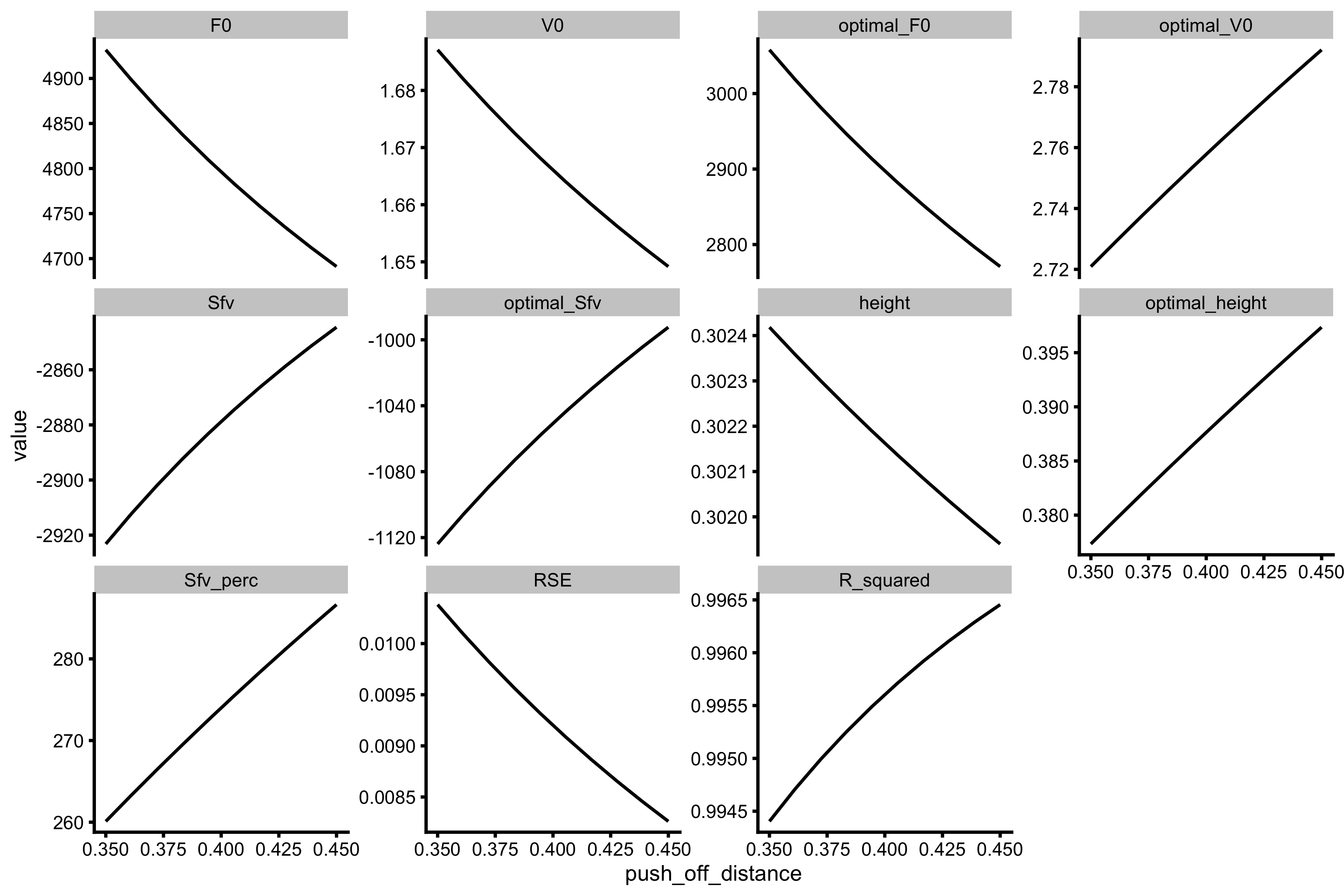
This procedure could be used as even “simpler” analysis than Samozino suggested. It is not perfect, but it can give some hints, particularly for \(S_{FV}\%\) metric.
Providing confidence intervals using bootstrap
Let’s write a function that returns Samozino model with 95% confidence intervals using bmbstats package (Jovanović 2020b, 2019, 2020a). bmbstats performs a bootstrap and returns the metrics (i.e., estimators). I have implemented one “trick” here to make bootstrap work, particularly for athletes with small number of observations (e.g., less than 5): I have create a strata vector. In this case strata has two compartments: high (all jump reps over over and equal to median total mass) and low (all jump reps under median total mass). This way we made sure that at least two different data points (from high vs. low load sets) will be available in each bootstrap resample which is needed to create a profile. For the sake of example, let’s give Chris a push-off distance of 0.4m, so we are able to estimate his Samozino metrics.
# Need to reload the data
data("testing_data")

# Impute missing value for Chris
testing_data[testing_data$athlete == "Chris", ]$push_off_distance <- 0.4

# Calculate mean GRF and mean Velocity
testing_data <- testing_data %>%
  mutate(height = vjsim::get_height_from_aerial_time(aerial_time)) %>%
  # Need to add bodyweight so it is kept in the output
  group_by(athlete, bodyweight) %>%
  do(jump_metric(.))

boot_samozino_profile <- function(data) {
  # Create boot strata to make sure at least two unique points are sampled
  data_strata <- factor(ifelse(data$mass < median(data$mass), "low", "high"))

  boot_data <- bmbstats::bmbstats(
    data = data,
    estimator_function = function(data, SESOI_lower, SESOI_upper, na.rm, init_boot) {
      samozino_data <- vjsim::get_samozino_profile(
        bodyweight = data$bodyweight,
        push_off_distance = data$push_off_distance,
        mean_GRF_over_distance = data$mean_GRF_over_distance,
        mean_velocity = data$mean_velocity
      )
      return(samozino_data)
    },
    control = model_control(
      boot_samples = 1000,
      confidence = 0.95,
      iter = FALSE,
      boot_type = "perc",
      boot_strata = data_strata
    )
  )

  return(boot_data$estimators)
}

testing_data_samozino <- testing_data %>%
  # Need to add bodyweight so it is kept in the output
  group_by(athlete, bodyweight) %>%
  do(boot_samozino_profile(.))

datatable(testing_data_samozino, rownames = FALSE) %>%
  formatRound(columns = 1:ncol(testing_data_samozino), digits = 2)
We can plot the bootstrapped estimates for each athlete:
ggplot(
  # Plot only selected metrics
  testing_data_samozino %>%
    filter(estimator %in% c("F0", "V0", "optimal_F0", "optimal_V0", "Sfv", "optimal_Sfv", "height", "optimal_height", "Sfv_perc", "RSE", "R_squared")) %>%
    mutate(estimator = factor(estimator, levels = c("F0", "V0", "optimal_F0", "optimal_V0", "Sfv", "optimal_Sfv", "height", "optimal_height", "Sfv_perc", "RSE", "R_squared"))),
  aes(y = athlete, x = value)
) +
  theme_bw(8) +
  geom_errorbarh(aes(xmax = upper, xmin = lower),
    color = "black",
    height = 0
  ) +
  geom_point() +
  xlab("") + ylab("") +
  facet_wrap(~estimator, scales = "free_x")
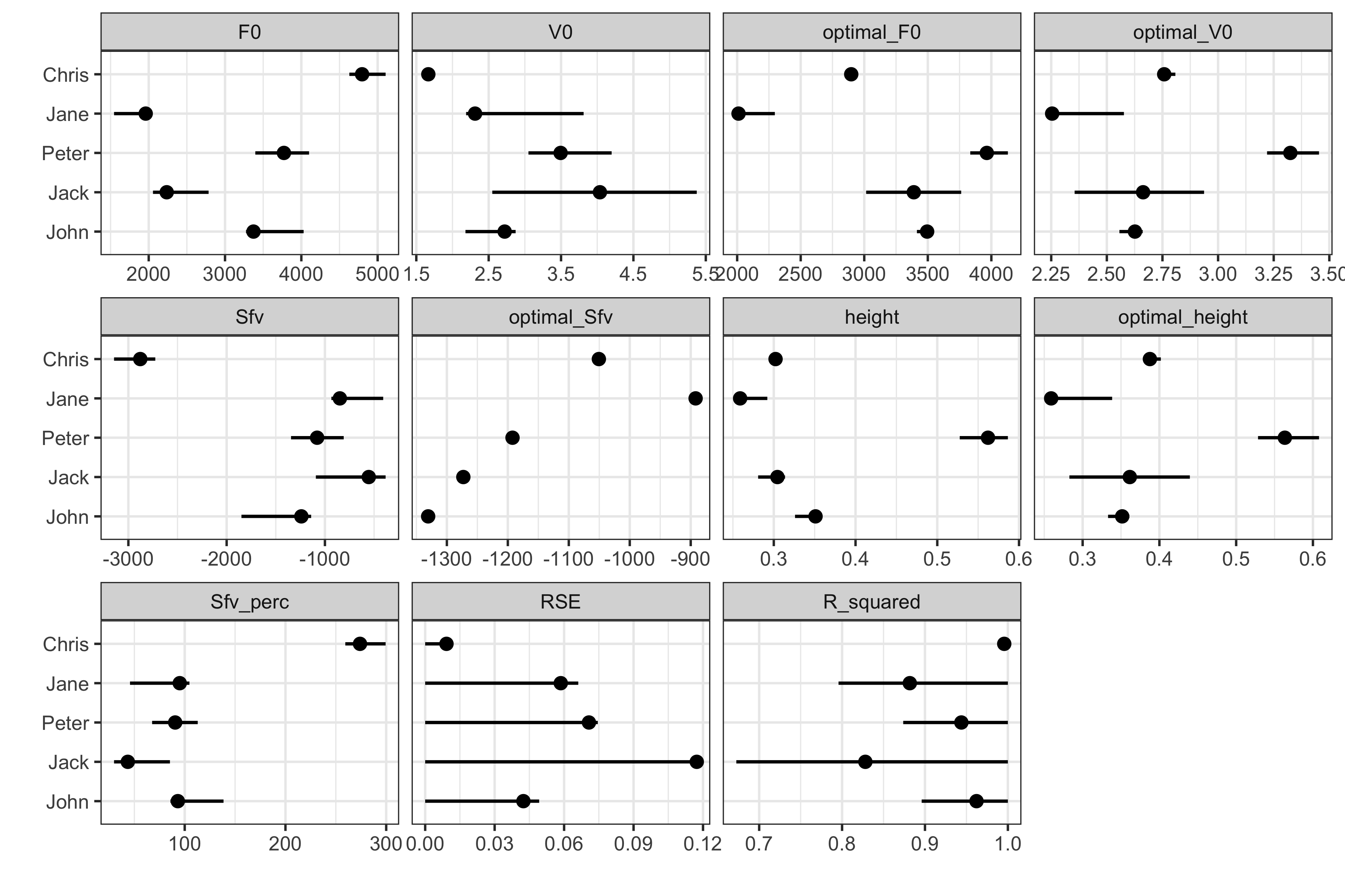
This figure can give us some idea about uncertainty around metrics. The more data collected, the more they fit on the straight line, the uncertainty will be lower. Take Chris for example (after we imputed the missing value of course): if you look at his FV profile, the shaded area around regression line is smallest (which means that the observations are less jumpy). This is reflected in shorter error bars in the above figure (i.e., uncertainty around metrics).
Dealing with know measurement errors
The analysis we perform assumes we are dealing with true values, without measurement error. Unfortunately, every measurement has some measurement error. We estimate these error (i.e. random error (RE); or measurement error variance) in a reliability study. Let’s assume that we know the measurement errors for the jump mat flight time (RE=0.01s), push-off distance (RE=0.01m), and bodyweight (RE=0.25kg). These error are already inside our observations (let’s call this error factor 1). How do we estimate our metrics as if there is no measurement error? How do we evaluate how the measurement error affect our estimates?
One technique that is very useful, although not often used in sport science practice and research, is called simulation extrapolation (SIMEX) (Keogh et al. 2020; Shaw et al. 2020; Wallace 2020). Using simulations, we can on purpose add (known) error of particular magnitude on observations (e.g. observation + 0.5xRE; which is equal to factor 1.5, since we already have error in our observations). Then we can extrapolate estimates to zero error (when error factor is 0).
Since this is simulation and might take a long time, I’ve used SIMEX only on one athlete, Jack (since he has the widest compatibility band around the FV profile). The code below is my implementation of the SIMEX. Each error factor is simulated 200 times.
# Need to reload the data
data("testing_data")

# Impute missing value for Chris
testing_data[testing_data$athlete == "Chris", ]$push_off_distance <- 0.4

# known measurement errors (hypothetical)
aerial_time_error <- 0.01
push_off_distance_error <- 0.01
bodyweight_error <- 0.250

testing_data_error <- expand_grid(
  testing_data,
  aerial_time_error = aerial_time_error,
  push_off_distance_error  = push_off_distance_error,
  bodyweight_error = bodyweight_error,
  error_factor = seq(1, 3, length.out = 5),
  rep = seq(1, 200)
)

SIMEX_samozino_profile <- function(data) {

  # Add error to data
  # Only one error to bodyweight and push-off distance, but multiple for aerial_time
  data <- data %>%
    mutate(
      bodyweight = bodyweight + rnorm(1, 0, bodyweight_error[1] * (error_factor[1] - 1)),
      push_off_distance = push_off_distance + rnorm(1, 0, push_off_distance_error * (error_factor - 1)),
      aerial_time = aerial_time + rnorm(n(), 0, aerial_time_error * (error_factor - 1))
    )

  # Calculate mean GRF and mean Velocity
  data <- data %>%
    mutate(height = vjsim::get_height_from_aerial_time(aerial_time)) %>%
    # Need to add bodyweight so it is kept in the output
    group_by(athlete, bodyweight) %>%
    do(jump_metric(.))

  samozino_data <- vjsim::get_samozino_profile(
    bodyweight = data$bodyweight,
    push_off_distance = data$push_off_distance,
    mean_GRF_over_distance = data$mean_GRF_over_distance,
    mean_velocity = data$mean_velocity
  )
  return(as.data.frame(samozino_data))
}

samozino_error_data <- testing_data_error %>%
  # Use only Jack
  filter(athlete == "Jack") %>%
  # Need to add bodyweight so it is kept in the output
  group_by(athlete, bodyweight, error_factor, rep) %>%
  do(SIMEX_samozino_profile(.))


datatable(samozino_error_data, rownames = FALSE) %>%
  formatRound(columns = 1:ncol(samozino_error_data), digits = 2)
Each simulation for each error factor can be depicted as a line. The average of those lines (or average of metric across simulation reps) is the estimate of the metric for a particular error factor. Here is the neat plot:
samozino_error_data_long <- gather(samozino_error_data, "metric", "value", -(1:4))

# Plot
ggplot(
  samozino_error_data_long %>%
    filter(metric %in% c("F0", "V0", "optimal_F0", "optimal_V0", "Sfv", "optimal_Sfv", "height", "optimal_height", "Sfv_perc", "RSE", "R_squared")) %>%
    mutate(metric = factor(metric, levels = c("F0", "V0", "optimal_F0", "optimal_V0", "Sfv", "optimal_Sfv", "height", "optimal_height", "Sfv_perc", "RSE", "R_squared"))),
  aes(x = error_factor, group = rep, y = value)
) +
  theme_cowplot(8) +
  geom_line(alpha = 0.1) +
  facet_wrap(~metric, scales = "free_y") +
  geom_vline(xintercept = 0, color = "transparent") +
  geom_smooth(group = 1, se = FALSE, method = "lm", formula = y ~ I(x^2), fullrange = TRUE, size = 0.5) +
  ylab(NULL) +
  ggtitle("Jack")
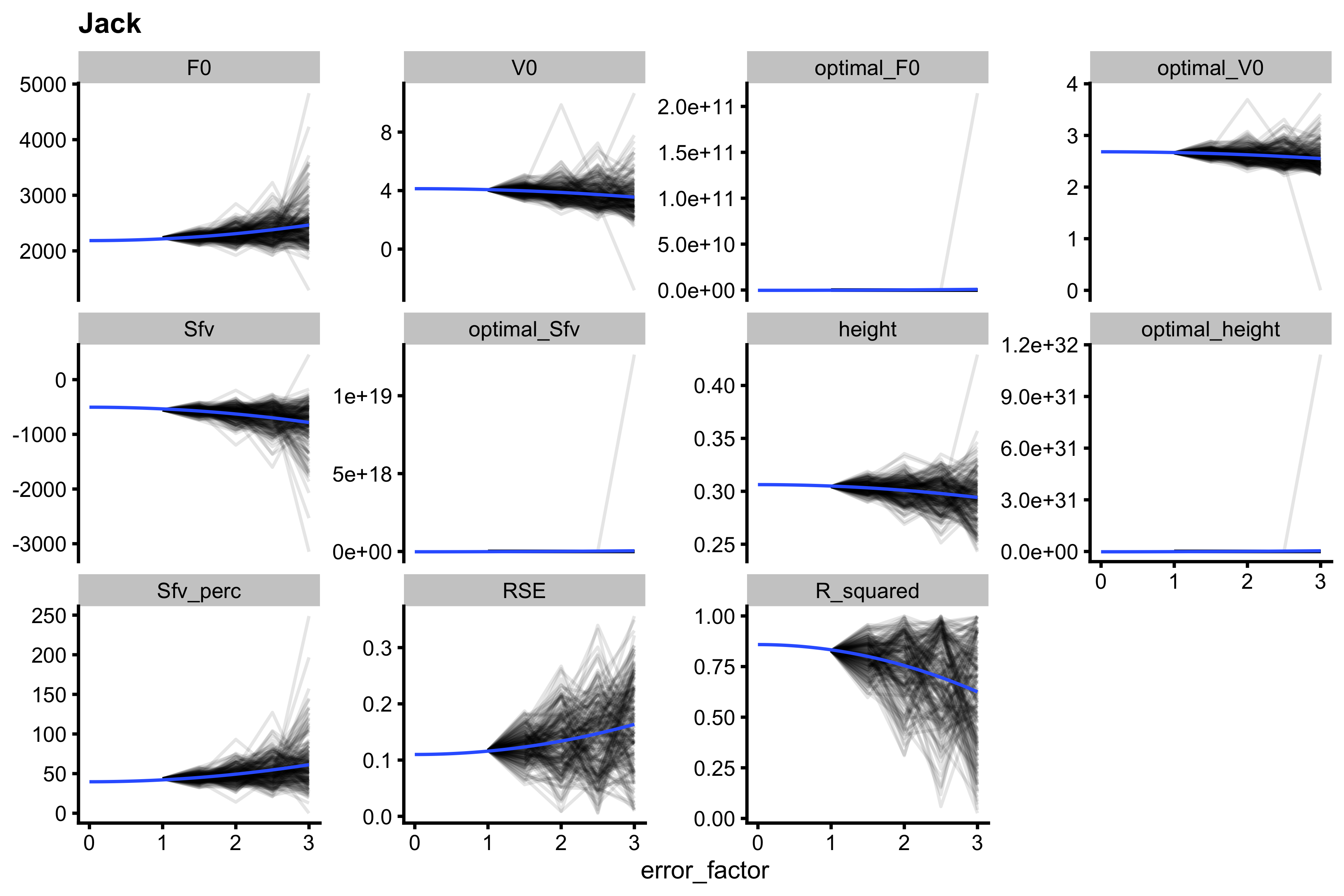
These averages are modeled with cubic linear regression, and this can be extrapolated to a error factor of 0, which indicates metric estimates when there is no error.
We can also provide confidence limits for each simulation and summarize those as well, but that can take tremendous computing time since we need to do bootstrap for each athlete, each error factor and each simulation. It is thus not considered here.
SIMEX represent very useful analysis technique since it allows us to take into account the know measurement errors. I will leave you to play with the code and explore how different measurement errors affect the metric estimates for John (or any other athlete).
Conclusion
Hopefully the functions from vjsim, particularly those used in this modeling vignette, can be useful in practice and might help researches and coaches develop squat jump profiles, but this time with addition of uncertainty intervals and SIMEX analysis.
Addendum
Package vjsim also has two functions that simplify profile building using the data collected: vjsim::make_samozino_profile and vjsim::make_load_profile. Let’s explore vjsim::make_samozino_profile first using the testing_data:
data("testing_data")

with(
  filter(testing_data, athlete == "Jack"),
  make_samozino_profile(
    bodyweight = bodyweight,
    push_off_distance = push_off_distance,
    external_load = external_load,
    aerial_time = aerial_time,
    plot = TRUE
  )
)
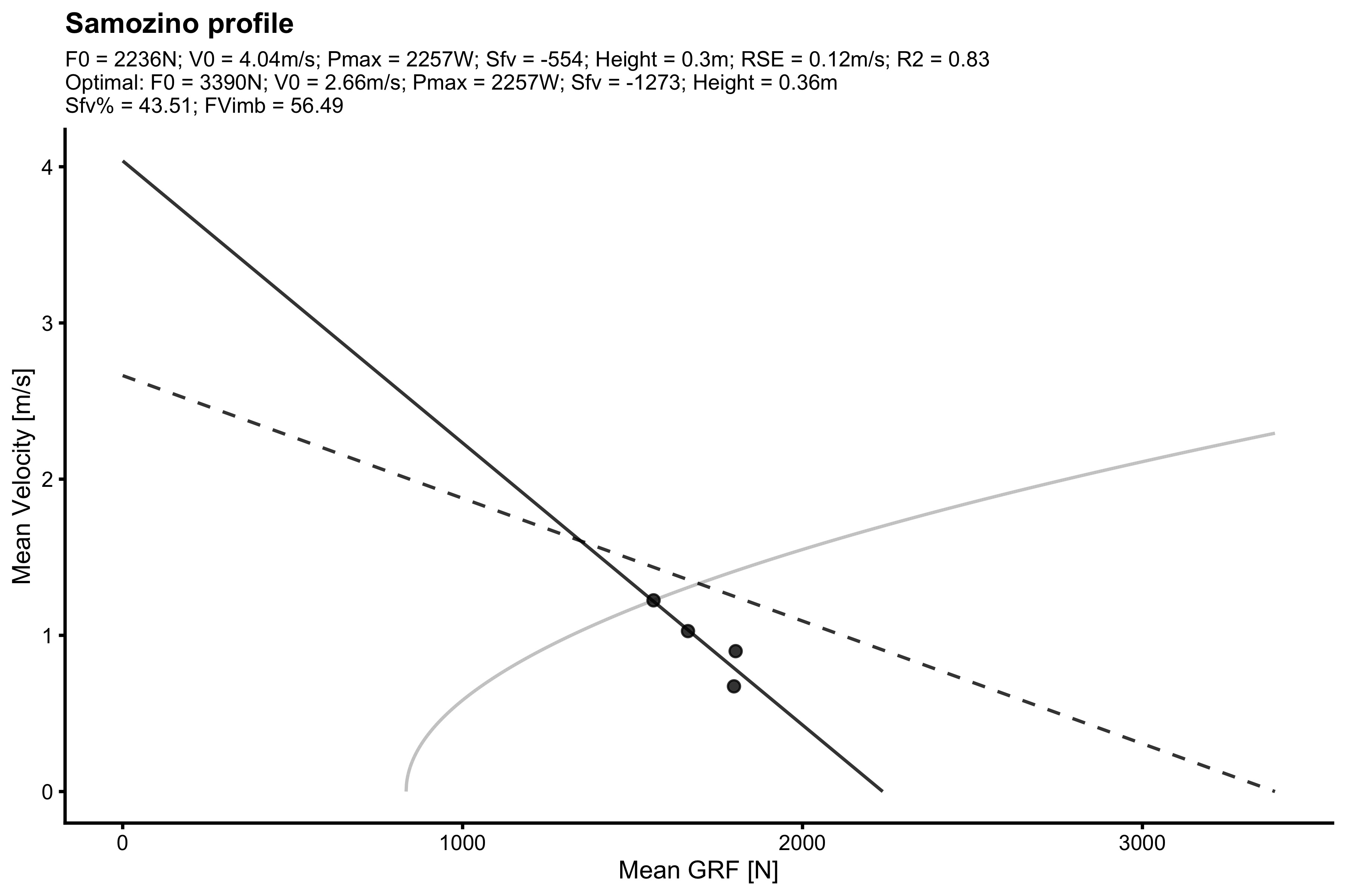
#> $F0
#> [1] 2235.995
#>
#> $F0_rel
#> [1] 26.30583
#>
#> $V0
#> [1] 4.037337
#>
#> $Pmax
#> [1] 2256.867
#>
#> $Pmax_rel
#> [1] 26.55137
#>
#> $Sfv
#> [1] -553.8293
#>
#> $Sfv_rel
#> [1] -6.515638
#>
#> $take_off_velocity
#> [1] 2.444065
#>
#> $height
#> [1] 0.3044574
#>
#> $optimal_F0
#> [1] 3389.95
#>
#> $optimal_F0_rel
#> [1] 39.88176
#>
#> $optimal_V0
#> [1] 2.663009
#>
#> $optimal_height
#> [1] 0.3614484
#>
#> $optimal_height_diff
#> [1] 0.05699097
#>
#> $optimal_height_ratio
#> [1] 1.187189
#>
#> $optimal_Pmax
#> [1] 2256.867
#>
#> $optimal_Pmax_rel
#> [1] 26.55137
#>
#> $optimal_take_off_velocity
#> [1] 2.663009
#>
#> $optimal_take_off_velocity_diff
#> [1] 0.2189439
#>
#> $optimal_take_off_velocity_ratio
#> [1] 1.089582
#>
#> $optimal_Sfv
#> [1] -1272.977
#>
#> $optimal_Sfv_rel
#> [1] -14.9762
#>
#> $Sfv_perc
#> [1] 43.50661
#>
#> $FV_imbalance
#> [1] 56.49339
#>
#> $probe_IMB
#> [1] 42.45125
#>
#> $RSE
#> [1] 0.1172931
#>
#> $R_squared
#> [1] 0.8280585
Function vjsim::make_samozino_profile thus provides all the modeling explained in this vignette in one command, and spits out the Samozino profile parameters, as well as create a neat summary graph.
Function vjsim::make_load_profile does the same functionality, but generated Load-TOV profile.
with(
  filter(testing_data, athlete == "Jack"),
  make_load_profile(
    bodyweight = bodyweight,
    external_load = external_load,
    aerial_time = aerial_time,
    plot = TRUE
  )
)
#> $L0
#> [1] 222.3918
#>
#> $L0_rel
#> [1] 2.616374
#>
#> $TOV0
#> [1] 3.959045
#>
#> $Sltv
#> [1] -56.17309
#>
#> $Sltv_rel
#> [1] -0.6608599
#>
#> $RSE
#> [1] 0.0560288
#>
#> $R_squared
#> [1] 0.9901916
If you want to provide profile summaries for multiple athletes using dplyr and tidyverse, use the following wrapper:
make_samozino_profile_wrapper <- function(data) {
  profile <- with(
    data,
    make_samozino_profile(
      bodyweight = bodyweight,
      push_off_distance = push_off_distance,
      external_load = external_load,
      aerial_time = aerial_time,
      plot = FALSE
    )
  )

  return(data.frame(
    F0 = profile$F0,
    V0 = profile$V0,
    height = profile$height,
    optimal_F0 = profile$optimal_F0,
    optimal_V0 = profile$optimal_V0,
    optimal_height = profile$optimal_height,
    Sfv_perc = profile$Sfv_perc
  ))
}

athlete_profiles <- testing_data %>%
  group_by(athlete) %>%
  do(make_samozino_profile_wrapper(.))


athlete_profiles
#> # A tibble: 5 x 8
#> # Groups:   athlete [5]
#>   athlete    F0    V0 height optimal_F0 optimal_V0 optimal_height Sfv_perc
#>   <fct>   <dbl> <dbl>  <dbl>      <dbl>      <dbl>          <dbl>    <dbl>
#> 1 John    3373.  2.72  0.351      3495.       2.63          0.352     93.2
#> 2 Jack    2236.  4.04  0.304      3390.       2.66          0.361     43.5
#> 3 Peter   3772.  3.49  0.562      3964.       3.32          0.563     90.5
#> 4 Jane    1961.  2.31  0.259      2011.       2.25          0.259     95.1
#> 5 Chris     NA  NA    NA            NA       NA            NA         NA
These two functions provide simple way you can analyze your own jump squat data.
References
Jovanović, Mladen. 2020a. Bmbstats: Bootstrap Magnitude-Based Statistics. https://github.com/mladenjovanovic/bmbstats.
———. 2020b. “Bmbstats: Magnitude-Based Statistics for Sports Scientists.” https://mladenjovanovic.github.io/bmbstats-book/. https://mladenjovanovic.github.io/bmbstats-book/.
———. 2019. “Statistical Modelling for Sports Scientists: Practical Introduction Using R (Part 1).” SportRxiv, September. https://doi.org/10.31236/osf.io/dnq3m.
Keogh, Ruth H., Pamela A. Shaw, Paul Gustafson, Raymond J. Carroll, Veronika Deffner, Kevin W. Dodd, Helmut Küchenhoff, et al. 2020. “STRATOS Guidance Document on Measurement Error and Misclassification of Variables in Observational Epidemiology: Part 1-Basic Theory and Simple Methods of Adjustment.” Statistics in Medicine, April. https://doi.org/10.1002/sim.8532.
Samozino, Pierre. 2018. “A Simple Method for Measuring Lower Limb Force, Velocity and Power Capabilities During Jumping.” In Biomechanics of Training and Testing, edited by Jean-Benoit Morin and Pierre Samozino, 65–96. Cham: Springer International Publishing. https://doi.org/10.1007/978-3-319-05633-3_4.
Samozino, Pierre, Jean-Benoît Morin, Frédérique Hintzy, and Alain Belli. 2008. “A Simple Method for Measuring Force, Velocity and Power Output During Squat Jump.” Journal of Biomechanics 41 (14): 2940–5. https://doi.org/10.1016/j.jbiomech.2008.07.028.
Samozino, Pierre, Jean-Benoît Morin, Frédérique Hintzy, and Alain Belli. 2010. “Jumping Ability: A Theoretical Integrative Approach.” Journal of Theoretical Biology 264 (1): 11–18. https://doi.org/10.1016/j.jtbi.2010.01.021.
Shaw, Pamela A., Paul Gustafson, Raymond J. Carroll, Veronika Deffner, Kevin W. Dodd, Ruth H. Keogh, Victor Kipnis, et al. 2020. “STRATOS Guidance Document on Measurement Error and Misclassification of Variables in Observational Epidemiology: Part 2-More Complex Methods of Adjustment and Advanced Topics.” Statistics in Medicine, April. https://doi.org/10.1002/sim.8531.
Wallace, Michael. 2020. “Analysis in an Imperfect World.” Significance 17 (1): 14–19. https://doi.org/10.1111/j.1740-9713.2020.01353.x.
I am watching my language here since it is very easy to make some stupid statements when discussing confidence intervals.↩︎