This function plots the selected estimator
# S3 method for athletemonitoring
plot(x, type = "line", ...)
Arguments
- x
Object of class
athletemonitoring- type
Type of the graph. Use "bar", "calendar", "table" or "line" (default). See Examples
- ...
Extra arguments. See Examples
Examples
# Load monitoring data set
data("monitoring")
# Filter out only 'Training Load'
monitoring <- monitoring[monitoring$Variable == "Training Load", ]
# Convert column to date format (or use numeric)
monitoring$Date <- as.Date(monitoring$Date, "%Y-%m-%d")
# Run the athlete monitoring data preparation
prepared_data <- prepare(
data = monitoring,
athlete = "Full Name",
date = "Date",
variable = "Variable",
value = "Value",
acute = 7,
chronic = 42,
# How should be missing entry treated?
# What do we assume? Zero load? Let's keep NA
NA_session = NA,
# How should missing days (i.e. no entries) be treated?
# Here we assume no training, hence zero
NA_day = 0,
# How should be multiple day entries summarised?
# With "load", it is a "sum", witho other metrics that
# do not aggregate, it can me "mean"
day_aggregate = function(x) {
sum(x, na.rm = TRUE)
},
# Rolling estimators for Acute and Chronic windows
rolling_estimators = function(x) {
c(
"mean" = mean(x, na.rm = TRUE),
"sd" = sd(x, na.rm = TRUE),
"cv" = sd(x, na.rm = TRUE) / mean(x, na.rm = TRUE)
)
},
# Additional estimator post-rolling
posthoc_estimators = function(data) {
data$ACD <- data$acute.mean - data$chronic.mean
data$ACR <- data$acute.mean / data$chronic.mean
data$ES <- data$ACD / data$chronic.sd
# Make sure to return the data
return(data)
},
# Group summary estimators
group_summary_estimators = function(x) {
c(
"median" = median(x, na.rm = TRUE),
"lower" = quantile(x, 0.25, na.rm = TRUE)[[1]],
"upper" = quantile(x, 0.75, na.rm = TRUE)[[1]]
)
}
)
#> Preparing data...
#> Rolling...
#> Group summaries...
#> Missing data summaries...
#> Done!
# Get summary
prepared_data
#> Athlete monitoring numeric data with the following characteristics:
#>
#> 10 athletes:
#> Alan McDonald, Ann Whitaker, Eve Black, Frank West, John Doe, Michael Peterson, Mike Smith, Peter Jackson, Stuart Rogan, Susan Kane
#>
#> 363 days:
#> From 18263 to 18625
#>
#> 5200 total entries
#>
#> 0 missing entries
#> 510 missing days
#> 0 extended days
#>
#> 1 variables:
#> Training Load
#>
#> 10 estimators:
#> variable.value, acute.mean, acute.sd, acute.cv, chronic.mean, chronic.sd, chronic.cv, ACD, ACR, ES
summary(prepared_data)
#> # A tibble: 10 × 16
#> athlete variable `Total entries` `Day entries` `Missing entries`
#> <chr> <chr> <dbl> <int> <dbl>
#> 1 Alan McDonald Training Lo… 520 363 0
#> 2 Ann Whitaker Training Lo… 520 363 0
#> 3 Eve Black Training Lo… 520 363 0
#> 4 Frank West Training Lo… 520 363 0
#> 5 John Doe Training Lo… 520 363 0
#> 6 Michael Peterson Training Lo… 520 363 0
#> 7 Mike Smith Training Lo… 520 363 0
#> 8 Peter Jackson Training Lo… 520 363 0
#> 9 Stuart Rogan Training Lo… 520 363 0
#> 10 Susan Kane Training Lo… 520 363 0
#> # ℹ 11 more variables: `Missing days` <int>, `Extended days` <int>,
#> # `Start date` <dbl>, `Stop date` <dbl>, Mean <dbl>, SD <dbl>, Min <dbl>,
#> # Max <dbl>, Median <dbl>, IQR <dbl>, MAD <dbl>
## Plots
# Table plot
# Produces formattable output with sparklines
plot(
prepared_data,
type = "table",
# Use to filter out estimators
estimator_name = c("acute.mean", "chronic.mean", "ES", "chronic.sd", "chronic.cv"),
# Use to filter out athlete
# athlete_name = NULL,
# Use to filter out variables
# variable_name = NULL,
# Show last entries
last_n = 42,
# Round numbers
digits = 2
)
# Bar plot
# To plot group average
plot(
prepared_data,
type = "bar"
)
#> Plotting average across athletes. Please select athlete or use `trellis=TRUE`
#> Warning: Removed 42 rows containing missing values or values outside the scale range
#> (`geom_line()`).
#> Warning: Removed 42 rows containing missing values or values outside the scale range
#> (`geom_line()`).
 # To plot per athlete, use trellis argument
plot(
prepared_data,
type = "bar",
trellis = TRUE
)
#> Warning: Removed 420 rows containing missing values or values outside the scale range
#> (`geom_line()`).
#> Warning: Removed 420 rows containing missing values or values outside the scale range
#> (`geom_line()`).
# To plot per athlete, use trellis argument
plot(
prepared_data,
type = "bar",
trellis = TRUE
)
#> Warning: Removed 420 rows containing missing values or values outside the scale range
#> (`geom_line()`).
#> Warning: Removed 420 rows containing missing values or values outside the scale range
#> (`geom_line()`).
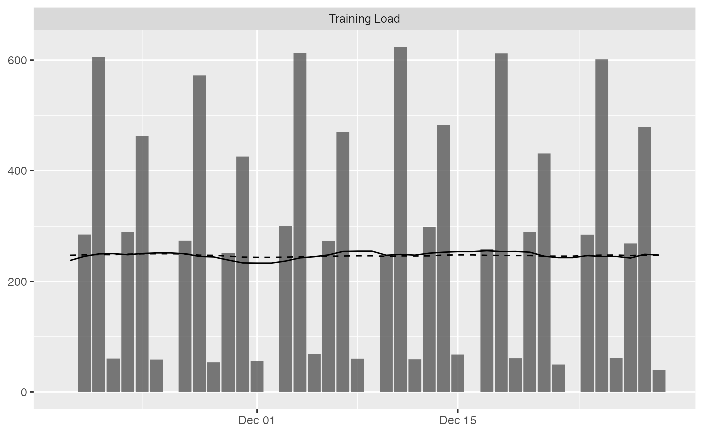
 # To filter out athletem variable and add Acute and Chronic lines to the group average:
plot(
prepared_data,
type = "bar",
# To filter out athletes
# athlete_name = NULL,
# To filter out variable
# variable_name = NULL,
# Add acute mean
acute_name = "acute.mean",
# Add chronic mean
chronic_name = "chronic.mean",
# Plot last n entries/days
last_n = 42
)
#> Plotting average across athletes. Please select athlete or use `trellis=TRUE`
# To filter out athletem variable and add Acute and Chronic lines to the group average:
plot(
prepared_data,
type = "bar",
# To filter out athletes
# athlete_name = NULL,
# To filter out variable
# variable_name = NULL,
# Add acute mean
acute_name = "acute.mean",
# Add chronic mean
chronic_name = "chronic.mean",
# Plot last n entries/days
last_n = 42
)
#> Plotting average across athletes. Please select athlete or use `trellis=TRUE`
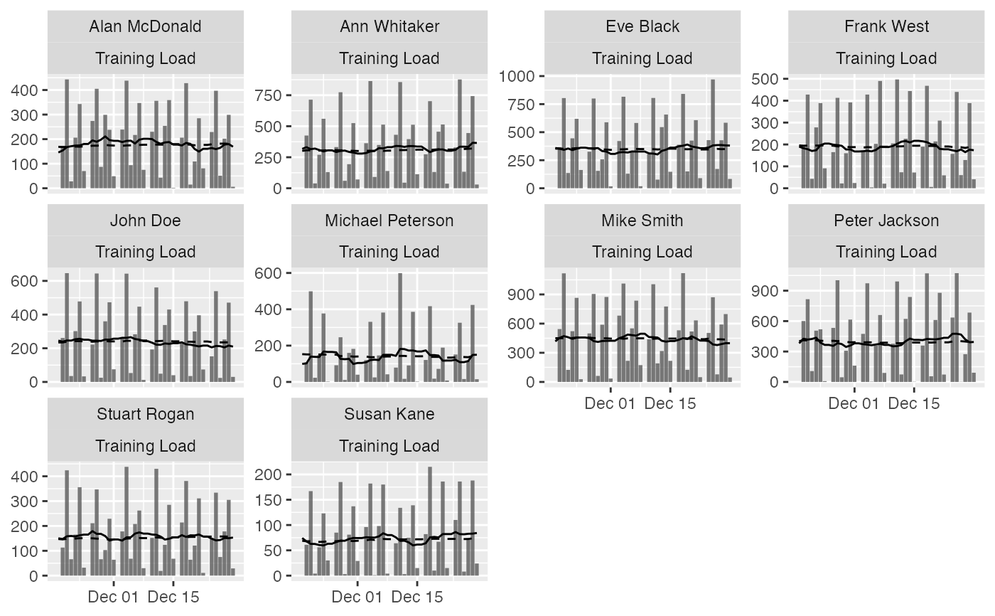
 # If you want to plot for each athlete, use trellis=TRUE
plot(
prepared_data,
type = "bar",
acute_name = "acute.mean",
chronic_name = "chronic.mean",
last_n = 42,
trellis = TRUE
)
# If you want to plot for each athlete, use trellis=TRUE
plot(
prepared_data,
type = "bar",
acute_name = "acute.mean",
chronic_name = "chronic.mean",
last_n = 42,
trellis = TRUE
)
 # Line plots
# These plots represent summary of the rollins estimators
plot(
prepared_data,
type = "line",
# To filter out athletes
# athlete_name = NULL,
# To filter out variables
# variable_name = NULL,
# To filter out estimators
# estimator_name = NULL,
# Tell graph where the lower group estimator is
# which is in this case 25%th percentile of the group
group_lower_name = "group.lower",
# The name of the centrality estimator of the group
group_central_name = "group.median",
# Tell graph where the upper group estimator is
# which is in this case 75%th percentile of the group
group_upper_name = "group.upper",
# Use trellis if you do not plot for a single individual
trellis = TRUE
)
# Line plots
# These plots represent summary of the rollins estimators
plot(
prepared_data,
type = "line",
# To filter out athletes
# athlete_name = NULL,
# To filter out variables
# variable_name = NULL,
# To filter out estimators
# estimator_name = NULL,
# Tell graph where the lower group estimator is
# which is in this case 25%th percentile of the group
group_lower_name = "group.lower",
# The name of the centrality estimator of the group
group_central_name = "group.median",
# Tell graph where the upper group estimator is
# which is in this case 75%th percentile of the group
group_upper_name = "group.upper",
# Use trellis if you do not plot for a single individual
trellis = TRUE
)
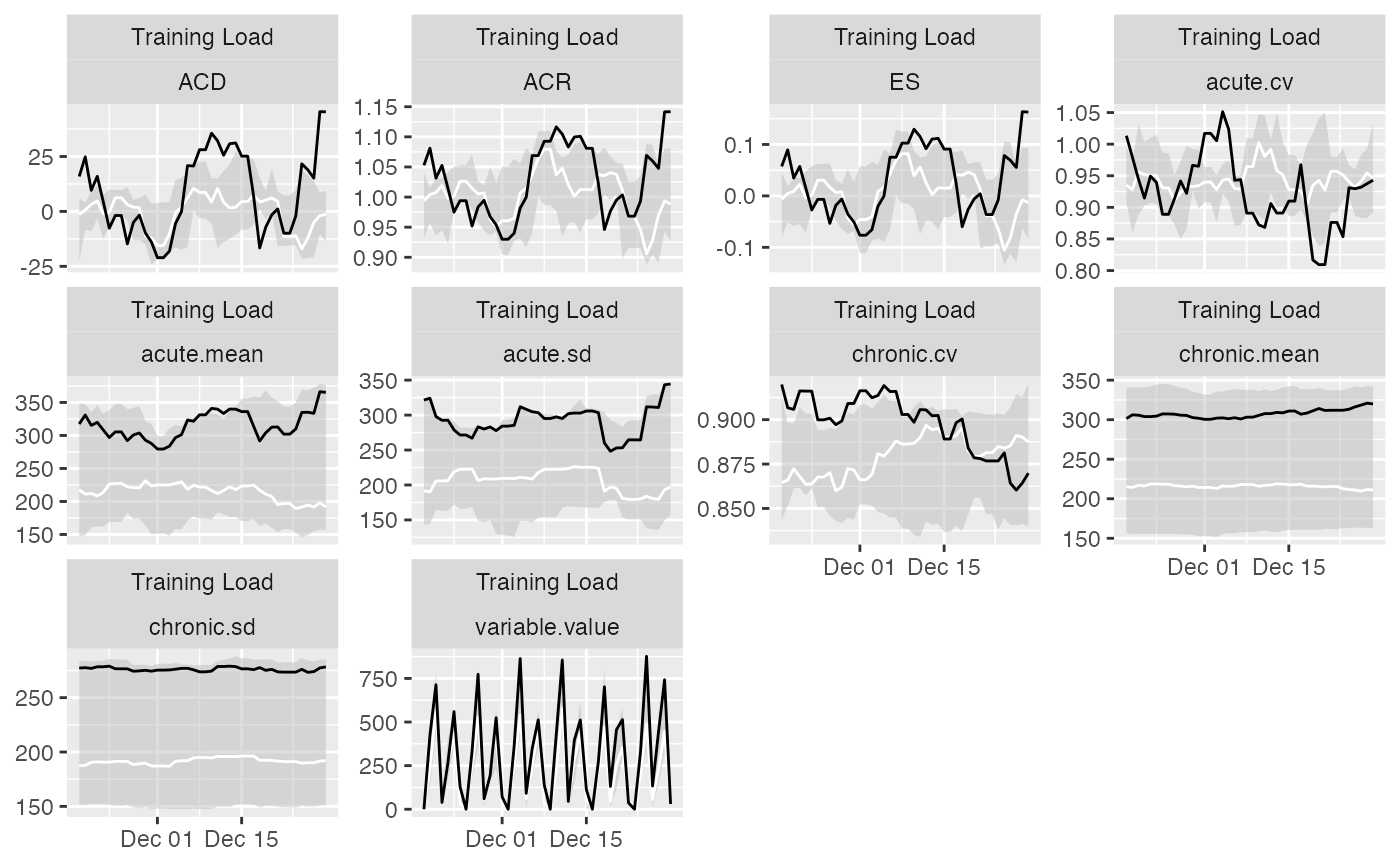
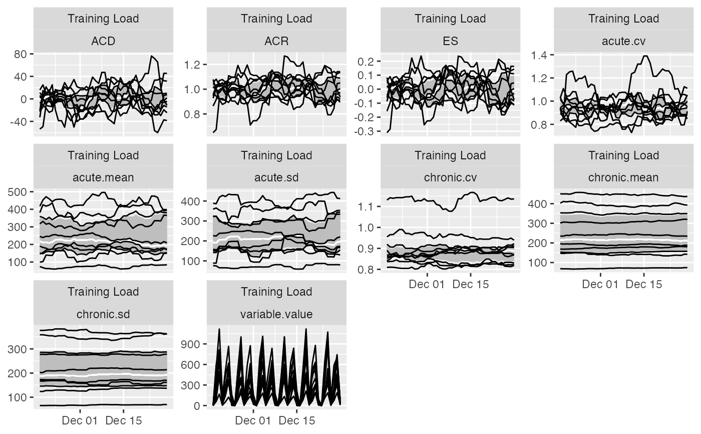 # Previous chart looks messy because it plot all athletes
# To avoid that, filter out only one athlete
plot(
prepared_data,
type = "line",
# To filter out athletes
athlete_name = "Ann Whitaker",
group_lower_name = "group.lower",
group_central_name = "group.median",
group_upper_name = "group.upper",
trellis = TRUE
)
# Previous chart looks messy because it plot all athletes
# To avoid that, filter out only one athlete
plot(
prepared_data,
type = "line",
# To filter out athletes
athlete_name = "Ann Whitaker",
group_lower_name = "group.lower",
group_central_name = "group.median",
group_upper_name = "group.upper",
trellis = TRUE
)
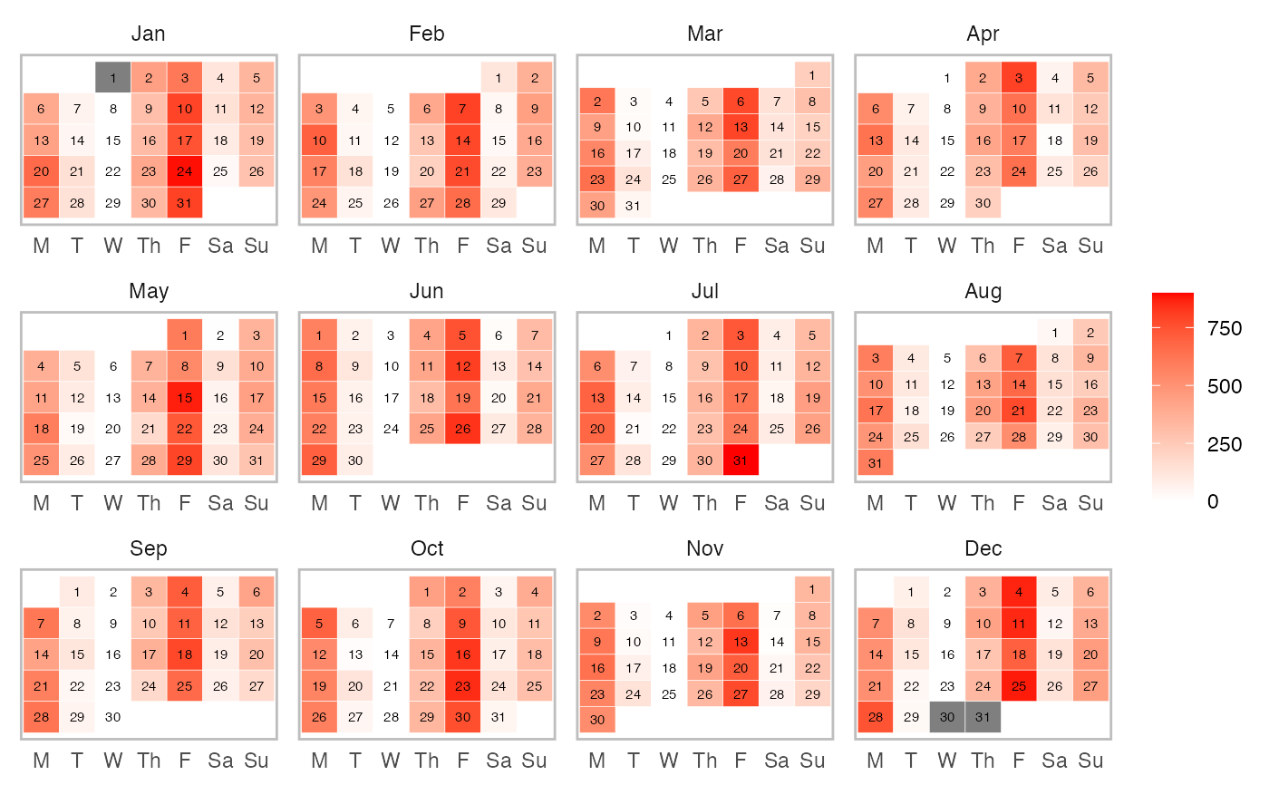
 # Calendar heatmap plot
plot(
prepared_data,
type = "calendar",
# To filter out athletes
athlete_name = "Ann Whitaker",
# To filter out variables
variable_name = "Training Load",
# To print estimator
estimator_name = "variable.value", # Or use "entries"
# To filter out last days
last_n = 365,
# To setup colors
low_color = "white",
high_color = "red",
na_color = "grey50",
# Should the whole year be plotted?
# Otherwise full months are plotted
full_year = FALSE,
# Should year label be plotted?
# in the case of multiple years involved
# it is always plotted
year_label = FALSE,
# Short weekdays?
short_weekday = TRUE,
# Label size
label_size = 2,
# Aggregation function in the case multiple athletes/variables/levels are used
aggregate_func = mean
)
# Calendar heatmap plot
plot(
prepared_data,
type = "calendar",
# To filter out athletes
athlete_name = "Ann Whitaker",
# To filter out variables
variable_name = "Training Load",
# To print estimator
estimator_name = "variable.value", # Or use "entries"
# To filter out last days
last_n = 365,
# To setup colors
low_color = "white",
high_color = "red",
na_color = "grey50",
# Should the whole year be plotted?
# Otherwise full months are plotted
full_year = FALSE,
# Should year label be plotted?
# in the case of multiple years involved
# it is always plotted
year_label = FALSE,
# Short weekdays?
short_weekday = TRUE,
# Label size
label_size = 2,
# Aggregation function in the case multiple athletes/variables/levels are used
aggregate_func = mean
)
 # Nominal data
# Create nominal variable
monitoring$Value_nominal <- cut(
monitoring$Value,
breaks = 5,
labels = c("Very Easy", "Easy", "Medium", "Hard", "Very Hard"),
include.lowest = TRUE
)
# Run the athlete monitoring data preparation
prepared_data <- prepare(
data = monitoring,
athlete = "Full Name",
date = "Date",
variable = "Variable",
value = "Value_nominal",
acute = 7,
chronic = 42,
# How should be missing entry treated?
NA_session = "<<<Session Missed>>>",
# How should missing days (i.e. no entries) be treated?
NA_day = "<<<Day Missed>>>",
# How should be multiple day entries summarised?
# This is different with levels, for example
# when there are two sessions, one is Low and one Hard
# if you use mean, then Low and Hard will be 0.5, with sum
# both will be 0.5, in which case the level probabilities will be
# summed to 1
day_aggregate = function(x) {
mean(x, na.rm = TRUE)
},
# Rolling estimators for Acute and Chronic windows
rolling_estimators = function(x) {
c(
"prop" = mean(x, na.rm = TRUE)
)
},
# Additional estimator post-rolling
posthoc_estimators = function(data) {
data$ACD <- data$acute.prop - data$chronic.prop
data$ACR <- data$acute.prop / data$chronic.prop
# Make sure to return the data
return(data)
},
# Group summary estimators
group_summary_estimators = function(x) {
c(
"median" = median(x, na.rm = TRUE),
"lower" = quantile(x, 0.25, na.rm = TRUE)[[1]],
"upper" = quantile(x, 0.75, na.rm = TRUE)[[1]]
)
}
)
#> Using nominal approach: column 'value' in the 'data' provided is not numeric. It will be treated as nominal and each level will be analyzed as separate variable using rolling counts approach.
#> Preparing data...
#> Rolling...
#> Group summaries...
#> Missing data summaries...
#> Done!
prepared_data
#> Athlete monitoring nominal data with the following characteristics:
#>
#> 10 athletes:
#> Alan McDonald, Ann Whitaker, Eve Black, Frank West, John Doe, Michael Peterson, Mike Smith, Peter Jackson, Stuart Rogan, Susan Kane
#>
#> 363 days:
#> From 18263 to 18625
#>
#> 34260 total entries
#>
#> 0 missing entries
#> 510 missing days
#> 0 extended days
#>
#> 1 variables:
#> Training Load
#>
#> 6 levels:
#> <<<Day Missed>>>, Easy, Hard, Medium, Very Easy, Very Hard
#>
#> 5 estimators:
#> variable.value, acute.prop, chronic.prop, ACD, ACR
summary(prepared_data)
#> # A tibble: 60 × 11
#> athlete variable level `Total entries` `Day entries` `Missing entries`
#> <chr> <chr> <chr> <int> <int> <dbl>
#> 1 Alan McDonald Training… <<<D… 571 363 0
#> 2 Alan McDonald Training… Easy 571 363 0
#> 3 Alan McDonald Training… Hard 571 363 0
#> 4 Alan McDonald Training… Medi… 571 363 0
#> 5 Alan McDonald Training… Very… 571 363 0
#> 6 Alan McDonald Training… Very… 571 363 0
#> 7 Ann Whitaker Training… <<<D… 571 363 0
#> 8 Ann Whitaker Training… Easy 571 363 0
#> 9 Ann Whitaker Training… Hard 571 363 0
#> 10 Ann Whitaker Training… Medi… 571 363 0
#> # ℹ 50 more rows
#> # ℹ 5 more variables: `Missing days` <int>, `Extended days` <int>,
#> # `Start date` <dbl>, `Stop date` <dbl>, Proportion <dbl>
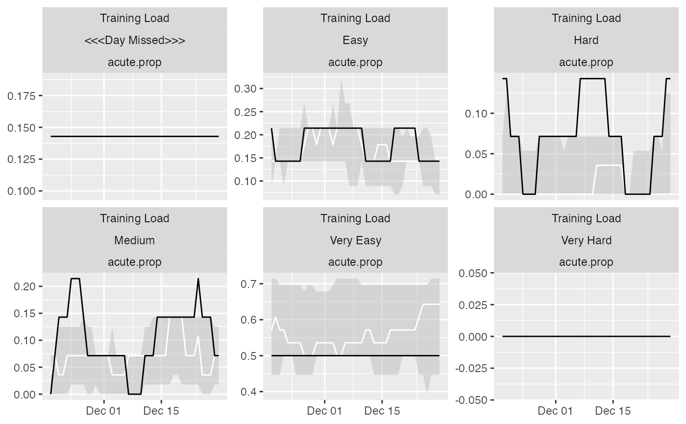
# Plots
plot(
prepared_data,
type = "line",
# To filter out athletes
athlete_name = "Ann Whitaker",
# To filter out variables
variable_name = "Training Load",
# To filter out estimators
estimator_name = "acute.prop",
group_lower_name = "group.lower",
group_central_name = "group.median",
group_upper_name = "group.upper",
trellis = TRUE
)
# Nominal data
# Create nominal variable
monitoring$Value_nominal <- cut(
monitoring$Value,
breaks = 5,
labels = c("Very Easy", "Easy", "Medium", "Hard", "Very Hard"),
include.lowest = TRUE
)
# Run the athlete monitoring data preparation
prepared_data <- prepare(
data = monitoring,
athlete = "Full Name",
date = "Date",
variable = "Variable",
value = "Value_nominal",
acute = 7,
chronic = 42,
# How should be missing entry treated?
NA_session = "<<<Session Missed>>>",
# How should missing days (i.e. no entries) be treated?
NA_day = "<<<Day Missed>>>",
# How should be multiple day entries summarised?
# This is different with levels, for example
# when there are two sessions, one is Low and one Hard
# if you use mean, then Low and Hard will be 0.5, with sum
# both will be 0.5, in which case the level probabilities will be
# summed to 1
day_aggregate = function(x) {
mean(x, na.rm = TRUE)
},
# Rolling estimators for Acute and Chronic windows
rolling_estimators = function(x) {
c(
"prop" = mean(x, na.rm = TRUE)
)
},
# Additional estimator post-rolling
posthoc_estimators = function(data) {
data$ACD <- data$acute.prop - data$chronic.prop
data$ACR <- data$acute.prop / data$chronic.prop
# Make sure to return the data
return(data)
},
# Group summary estimators
group_summary_estimators = function(x) {
c(
"median" = median(x, na.rm = TRUE),
"lower" = quantile(x, 0.25, na.rm = TRUE)[[1]],
"upper" = quantile(x, 0.75, na.rm = TRUE)[[1]]
)
}
)
#> Using nominal approach: column 'value' in the 'data' provided is not numeric. It will be treated as nominal and each level will be analyzed as separate variable using rolling counts approach.
#> Preparing data...
#> Rolling...
#> Group summaries...
#> Missing data summaries...
#> Done!
prepared_data
#> Athlete monitoring nominal data with the following characteristics:
#>
#> 10 athletes:
#> Alan McDonald, Ann Whitaker, Eve Black, Frank West, John Doe, Michael Peterson, Mike Smith, Peter Jackson, Stuart Rogan, Susan Kane
#>
#> 363 days:
#> From 18263 to 18625
#>
#> 34260 total entries
#>
#> 0 missing entries
#> 510 missing days
#> 0 extended days
#>
#> 1 variables:
#> Training Load
#>
#> 6 levels:
#> <<<Day Missed>>>, Easy, Hard, Medium, Very Easy, Very Hard
#>
#> 5 estimators:
#> variable.value, acute.prop, chronic.prop, ACD, ACR
summary(prepared_data)
#> # A tibble: 60 × 11
#> athlete variable level `Total entries` `Day entries` `Missing entries`
#> <chr> <chr> <chr> <int> <int> <dbl>
#> 1 Alan McDonald Training… <<<D… 571 363 0
#> 2 Alan McDonald Training… Easy 571 363 0
#> 3 Alan McDonald Training… Hard 571 363 0
#> 4 Alan McDonald Training… Medi… 571 363 0
#> 5 Alan McDonald Training… Very… 571 363 0
#> 6 Alan McDonald Training… Very… 571 363 0
#> 7 Ann Whitaker Training… <<<D… 571 363 0
#> 8 Ann Whitaker Training… Easy 571 363 0
#> 9 Ann Whitaker Training… Hard 571 363 0
#> 10 Ann Whitaker Training… Medi… 571 363 0
#> # ℹ 50 more rows
#> # ℹ 5 more variables: `Missing days` <int>, `Extended days` <int>,
#> # `Start date` <dbl>, `Stop date` <dbl>, Proportion <dbl>
# Plots
plot(
prepared_data,
type = "line",
# To filter out athletes
athlete_name = "Ann Whitaker",
# To filter out variables
variable_name = "Training Load",
# To filter out estimators
estimator_name = "acute.prop",
group_lower_name = "group.lower",
group_central_name = "group.median",
group_upper_name = "group.upper",
trellis = TRUE
)