Prepare Athlete Monitoring Data
prepare(
  data,
  athlete,
  date,
  variable,
  value,
  day_aggregate = function(x) {
     sum(x)
 },
  NA_session = NA,
  NA_day = NA,
  acute = 7,
  chronic = 28,
  partial = FALSE,
  rolling_fill = NA,
  rolling_estimators = function(x) {
     c(mean = mean(x, na.rm = TRUE), sd =
    stats::sd(x, na.rm = TRUE), cv = stats::sd(x, na.rm = TRUE)/mean(x, na.rm = TRUE),
    conf = sum(!is.na(x))/length(x))
 },
  posthoc_estimators = function(data) {
     return(data)
 },
  group_summary_estimators = function(x) {
     c(median = stats::median(x, na.rm =
    TRUE), lower = stats::quantile(x, 0.25, na.rm = TRUE)[[1]], upper =
    stats::quantile(x, 0.75, na.rm = TRUE)[[1]])
 },
  extend = c("none", "start", "end", "both"),
  extend_fill = NA_day,
  iter = TRUE
)
Arguments
- data
Data frame
- athlete
Name of the column in the
datawhere the athlete id or name is located- date
Name of the column in the
datawhere the date is located.datehas to be eitherDateornumericclass- variable
Name of the column in the
datawhere the variable name is located- value
Name of the column in the
datawhere the value ofvariableis located- day_aggregate
Function for aggregating multiple day entries. Defaults is
sum- NA_session
What value should be imputed for missing values in
value? Default isNA- NA_day
What value should be imputed for missing days? Default is
NA- acute
Duration of the acute rolling window. Default is 7
- chronic
Duration of the chronic rolling window. Default is 28
- partial
Logical or numeric. If
FALSE(default) thenrolling_estimatorsis only applied when all indexes of the rolling window are within the observed time range. IfTRUE, then the subset of indexes that are in range are passed torolling_estimators. A numeric argument to partial can be used to determine the minimal window size for partial computations.- rolling_fill
Value used to fill start of the rolling windows. Default is
NA- rolling_estimators
Function providing rolling estimators. See Details
- posthoc_estimators
Function providing post-hoc estimators. See Details
- group_summary_estimators
Function providing group summary estimators. See Details
- extend
Should all athletes, dates, and variables be aligned/extended to have all dates and levels. Default is
"none". Other options are"start"for aligning start dates,"end"for aligning end dates, and"both"for aligning both start and end days as well as variable levels across athletes- extend_fill
What value should be imputed for the extended days? Default is
NA_day- iter
Should progress be shown? Default is
TRUE
Value
Object of class athletemonitoring
Details
Extra arguments ... involve use_counts for nominal model
Examples
# Load monitoring data set
data("monitoring")
# Filter out only 'Training Load'
monitoring <- monitoring[monitoring$Variable == "Training Load", ]
# Convert column to date format (or use numeric)
monitoring$Date <- as.Date(monitoring$Date, "%Y-%m-%d")
# Run the athlete monitoring data preparation
prepared_data <- prepare(
data = monitoring,
athlete = "Full Name",
date = "Date",
variable = "Variable",
value = "Value",
acute = 7,
chronic = 42,
# How should be missing entry treated?
# What do we assume? Zero load? Let's keep NA
NA_session = NA,
# How should missing days (i.e. no entries) be treated?
# Here we assume no training, hence zero
NA_day = 0,
# How should be multiple day entries summarised?
# With "load", it is a "sum", witho other metrics that
# do not aggregate, it can me "mean"
day_aggregate = function(x) {
sum(x, na.rm = TRUE)
},
# Rolling estimators for Acute and Chronic windows
rolling_estimators = function(x) {
c(
"mean" = mean(x, na.rm = TRUE),
"sd" = sd(x, na.rm = TRUE),
"cv" = sd(x, na.rm = TRUE) / mean(x, na.rm = TRUE)
)
},
# Additional estimator post-rolling
posthoc_estimators = function(data) {
data$ACD <- data$acute.mean - data$chronic.mean
data$ACR <- data$acute.mean / data$chronic.mean
data$ES <- data$ACD / data$chronic.sd
# Make sure to return the data
return(data)
},
# Group summary estimators
group_summary_estimators = function(x) {
c(
"median" = median(x, na.rm = TRUE),
"lower" = quantile(x, 0.25, na.rm = TRUE)[[1]],
"upper" = quantile(x, 0.75, na.rm = TRUE)[[1]]
)
}
)
#> Preparing data...
#> Rolling...
#> Group summaries...
#> Missing data summaries...
#> Done!
# Get summary
prepared_data
#> Athlete monitoring numeric data with the following characteristics:
#>
#> 10 athletes:
#> Alan McDonald, Ann Whitaker, Eve Black, Frank West, John Doe, Michael Peterson, Mike Smith, Peter Jackson, Stuart Rogan, Susan Kane
#>
#> 363 days:
#> From 18263 to 18625
#>
#> 5200 total entries
#>
#> 0 missing entries
#> 510 missing days
#> 0 extended days
#>
#> 1 variables:
#> Training Load
#>
#> 10 estimators:
#> variable.value, acute.mean, acute.sd, acute.cv, chronic.mean, chronic.sd, chronic.cv, ACD, ACR, ES
summary(prepared_data)
#> # A tibble: 10 × 16
#> athlete variable `Total entries` `Day entries` `Missing entries`
#> <chr> <chr> <dbl> <int> <dbl>
#> 1 Alan McDonald Training Lo… 520 363 0
#> 2 Ann Whitaker Training Lo… 520 363 0
#> 3 Eve Black Training Lo… 520 363 0
#> 4 Frank West Training Lo… 520 363 0
#> 5 John Doe Training Lo… 520 363 0
#> 6 Michael Peterson Training Lo… 520 363 0
#> 7 Mike Smith Training Lo… 520 363 0
#> 8 Peter Jackson Training Lo… 520 363 0
#> 9 Stuart Rogan Training Lo… 520 363 0
#> 10 Susan Kane Training Lo… 520 363 0
#> # ℹ 11 more variables: `Missing days` <int>, `Extended days` <int>,
#> # `Start date` <dbl>, `Stop date` <dbl>, Mean <dbl>, SD <dbl>, Min <dbl>,
#> # Max <dbl>, Median <dbl>, IQR <dbl>, MAD <dbl>
## Plots
# Table plot
# Produces formattable output with sparklines
plot(
prepared_data,
type = "table",
# Use to filter out estimators
estimator_name = c("acute.mean", "chronic.mean", "ES", "chronic.sd", "chronic.cv"),
# Use to filter out athlete
# athlete_name = NULL,
# Use to filter out variables
# variable_name = NULL,
# Show last entries
last_n = 42,
# Round numbers
digits = 2
)
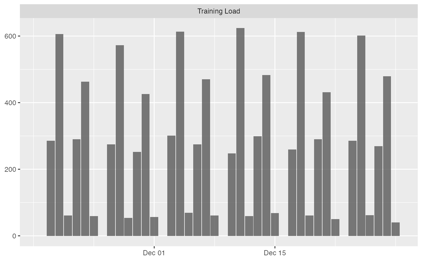
# Bar plot
# To plot group average
plot(
prepared_data,
type = "bar"
)
#> Plotting average across athletes. Please select athlete or use `trellis=TRUE`
#> Warning: Removed 42 rows containing missing values or values outside the scale range
#> (`geom_line()`).
#> Warning: Removed 42 rows containing missing values or values outside the scale range
#> (`geom_line()`).
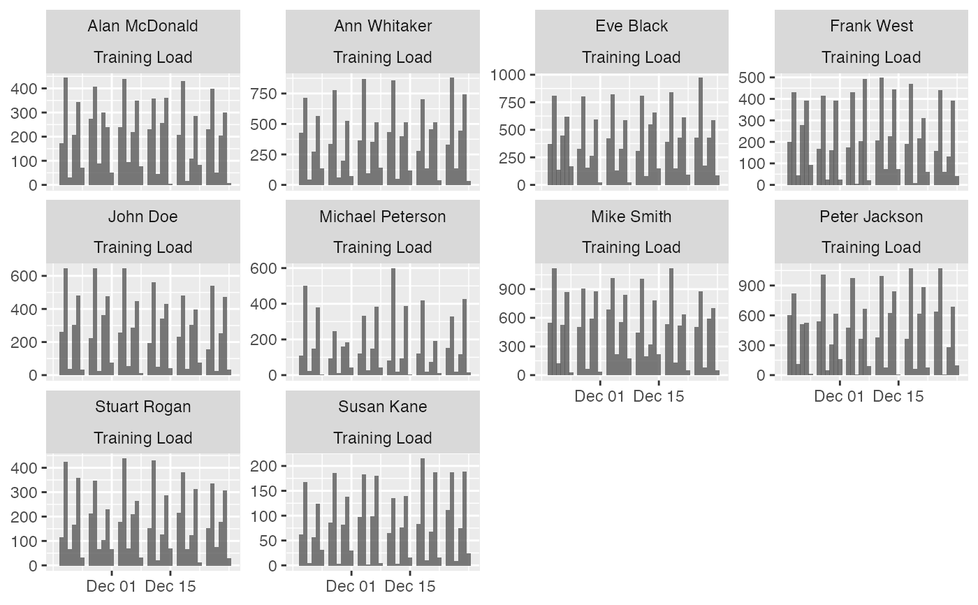
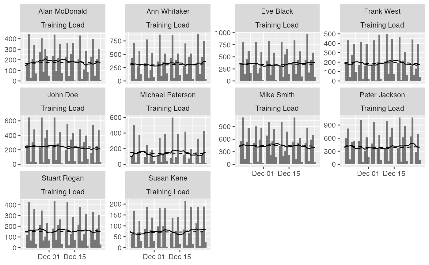
 # To plot per athlete, use trellis argument
plot(
prepared_data,
type = "bar",
trellis = TRUE
)
#> Warning: Removed 420 rows containing missing values or values outside the scale range
#> (`geom_line()`).
#> Warning: Removed 420 rows containing missing values or values outside the scale range
#> (`geom_line()`).
# To plot per athlete, use trellis argument
plot(
prepared_data,
type = "bar",
trellis = TRUE
)
#> Warning: Removed 420 rows containing missing values or values outside the scale range
#> (`geom_line()`).
#> Warning: Removed 420 rows containing missing values or values outside the scale range
#> (`geom_line()`).
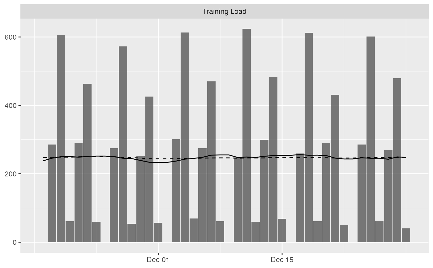
 # To filter out athletem variable and add Acute and Chronic lines to the group average:
plot(
prepared_data,
type = "bar",
# To filter out athletes
# athlete_name = NULL,
# To filter out variable
# variable_name = NULL,
# Add acute mean
acute_name = "acute.mean",
# Add chronic mean
chronic_name = "chronic.mean",
# Plot last n entries/days
last_n = 42
)
#> Plotting average across athletes. Please select athlete or use `trellis=TRUE`
# To filter out athletem variable and add Acute and Chronic lines to the group average:
plot(
prepared_data,
type = "bar",
# To filter out athletes
# athlete_name = NULL,
# To filter out variable
# variable_name = NULL,
# Add acute mean
acute_name = "acute.mean",
# Add chronic mean
chronic_name = "chronic.mean",
# Plot last n entries/days
last_n = 42
)
#> Plotting average across athletes. Please select athlete or use `trellis=TRUE`
 # If you want to plot for each athlete, use trellis=TRUE
plot(
prepared_data,
type = "bar",
acute_name = "acute.mean",
chronic_name = "chronic.mean",
last_n = 42,
trellis = TRUE
)
# If you want to plot for each athlete, use trellis=TRUE
plot(
prepared_data,
type = "bar",
acute_name = "acute.mean",
chronic_name = "chronic.mean",
last_n = 42,
trellis = TRUE
)
 # Line plots
# These plots represent summary of the rollins estimators
plot(
prepared_data,
type = "line",
# To filter out athletes
# athlete_name = NULL,
# To filter out variables
# variable_name = NULL,
# To filter out estimators
# estimator_name = NULL,
# Tell graph where the lower group estimator is
# which is in this case 25%th percentile of the group
group_lower_name = "group.lower",
# The name of the centrality estimator of the group
group_central_name = "group.median",
# Tell graph where the upper group estimator is
# which is in this case 75%th percentile of the group
group_upper_name = "group.upper",
# Use trellis if you do not plot for a single individual
trellis = TRUE
)
# Line plots
# These plots represent summary of the rollins estimators
plot(
prepared_data,
type = "line",
# To filter out athletes
# athlete_name = NULL,
# To filter out variables
# variable_name = NULL,
# To filter out estimators
# estimator_name = NULL,
# Tell graph where the lower group estimator is
# which is in this case 25%th percentile of the group
group_lower_name = "group.lower",
# The name of the centrality estimator of the group
group_central_name = "group.median",
# Tell graph where the upper group estimator is
# which is in this case 75%th percentile of the group
group_upper_name = "group.upper",
# Use trellis if you do not plot for a single individual
trellis = TRUE
)
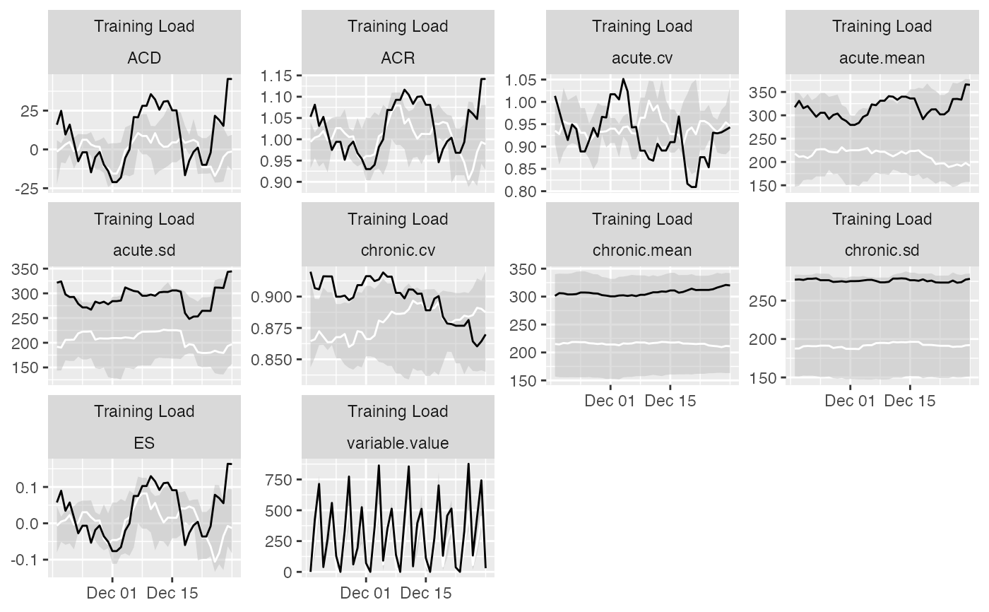
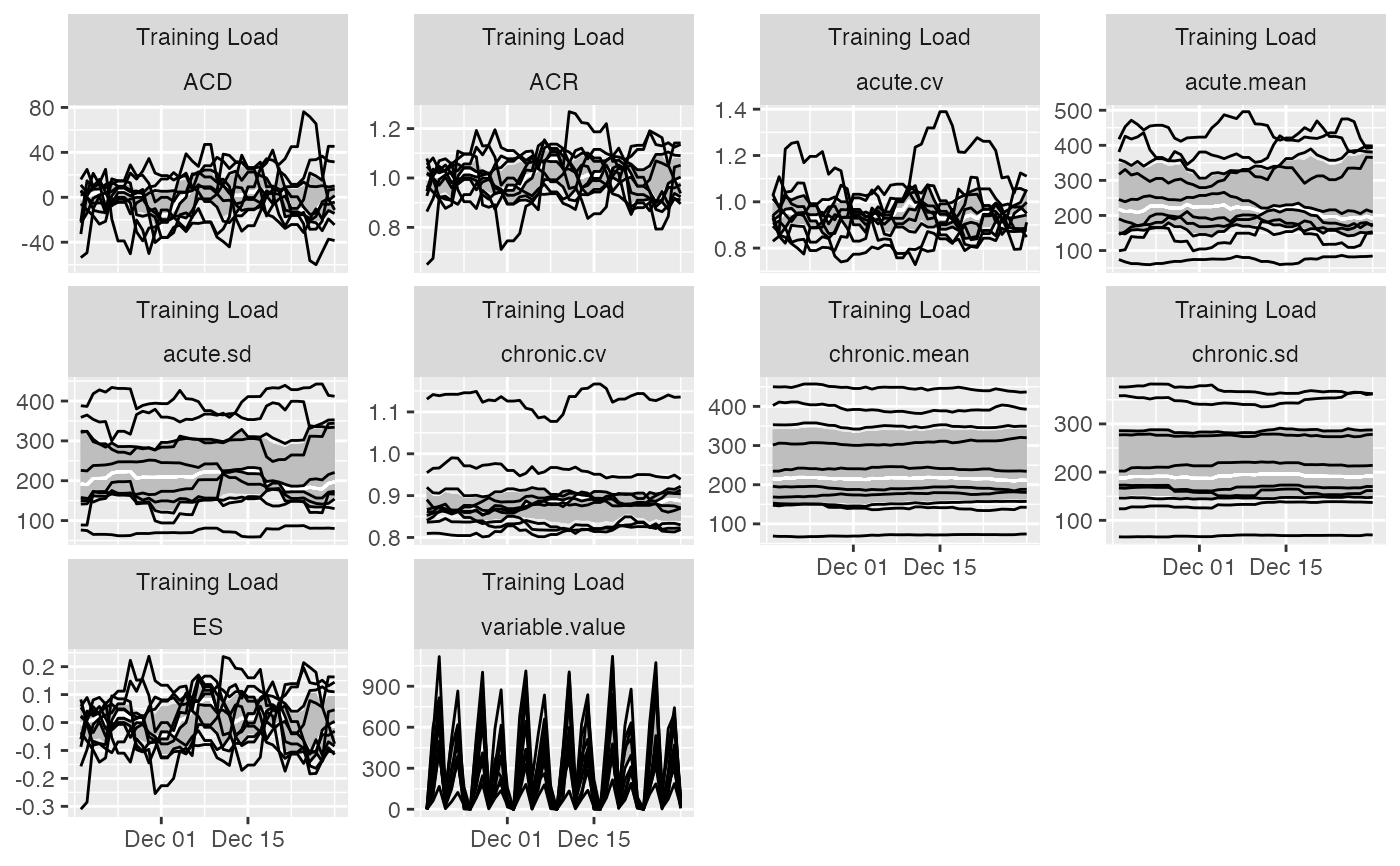 # Previous chart looks messy because it plot all athletes
# To avoid that, filter out only one athlete
plot(
prepared_data,
type = "line",
# To filter out athletes
athlete_name = "Ann Whitaker",
group_lower_name = "group.lower",
group_central_name = "group.median",
group_upper_name = "group.upper",
trellis = TRUE
)
# Previous chart looks messy because it plot all athletes
# To avoid that, filter out only one athlete
plot(
prepared_data,
type = "line",
# To filter out athletes
athlete_name = "Ann Whitaker",
group_lower_name = "group.lower",
group_central_name = "group.median",
group_upper_name = "group.upper",
trellis = TRUE
)
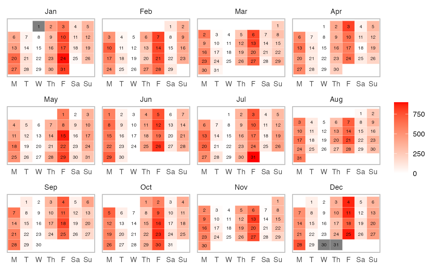
 # Calendar heatmap plot
plot(
prepared_data,
type = "calendar",
# To filter out athletes
athlete_name = "Ann Whitaker",
# To filter out variables
variable_name = "Training Load",
# To print estimator
estimator_name = "variable.value", # Or use "entries"
# To filter out last days
last_n = 365,
# To setup colors
low_color = "white",
high_color = "red",
na_color = "grey50",
# Should the whole year be plotted?
# Otherwise full months are plotted
full_year = FALSE,
# Should year label be plotted?
# in the case of multiple years involved
# it is always plotted
year_label = FALSE,
# Short weekdays?
short_weekday = TRUE,
# Label size
label_size = 2,
# Aggregation function in the case multiple athletes/variables/levels are used
aggregate_func = mean
)
# Calendar heatmap plot
plot(
prepared_data,
type = "calendar",
# To filter out athletes
athlete_name = "Ann Whitaker",
# To filter out variables
variable_name = "Training Load",
# To print estimator
estimator_name = "variable.value", # Or use "entries"
# To filter out last days
last_n = 365,
# To setup colors
low_color = "white",
high_color = "red",
na_color = "grey50",
# Should the whole year be plotted?
# Otherwise full months are plotted
full_year = FALSE,
# Should year label be plotted?
# in the case of multiple years involved
# it is always plotted
year_label = FALSE,
# Short weekdays?
short_weekday = TRUE,
# Label size
label_size = 2,
# Aggregation function in the case multiple athletes/variables/levels are used
aggregate_func = mean
)
 # Nominal data
# Create nominal variable
monitoring$Value_nominal <- cut(
monitoring$Value,
breaks = 5,
labels = c("Very Easy", "Easy", "Medium", "Hard", "Very Hard"),
include.lowest = TRUE
)
# Run the athlete monitoring data preparation
prepared_data <- prepare(
data = monitoring,
athlete = "Full Name",
date = "Date",
variable = "Variable",
value = "Value_nominal",
acute = 7,
chronic = 42,
# How should be missing entry treated?
NA_session = "<<<Session Missed>>>",
# How should missing days (i.e. no entries) be treated?
NA_day = "<<<Day Missed>>>",
# How should be multiple day entries summarised?
# This is different with levels, for example
# when there are two sessions, one is Low and one Hard
# if you use mean, then Low and Hard will be 0.5, with sum
# both will be 0.5, in which case the level probabilities will be
# summed to 1
day_aggregate = function(x) {
mean(x, na.rm = TRUE)
},
# Rolling estimators for Acute and Chronic windows
rolling_estimators = function(x) {
c(
"prop" = mean(x, na.rm = TRUE)
)
},
# Additional estimator post-rolling
posthoc_estimators = function(data) {
data$ACD <- data$acute.prop - data$chronic.prop
data$ACR <- data$acute.prop / data$chronic.prop
# Make sure to return the data
return(data)
},
# Group summary estimators
group_summary_estimators = function(x) {
c(
"median" = median(x, na.rm = TRUE),
"lower" = quantile(x, 0.25, na.rm = TRUE)[[1]],
"upper" = quantile(x, 0.75, na.rm = TRUE)[[1]]
)
}
)
#> Using nominal approach: column 'value' in the 'data' provided is not numeric. It will be treated as nominal and each level will be analyzed as separate variable using rolling counts approach.
#> Preparing data...
#> Rolling...
#> Group summaries...
#> Missing data summaries...
#> Done!
prepared_data
#> Athlete monitoring nominal data with the following characteristics:
#>
#> 10 athletes:
#> Alan McDonald, Ann Whitaker, Eve Black, Frank West, John Doe, Michael Peterson, Mike Smith, Peter Jackson, Stuart Rogan, Susan Kane
#>
#> 363 days:
#> From 18263 to 18625
#>
#> 34260 total entries
#>
#> 0 missing entries
#> 510 missing days
#> 0 extended days
#>
#> 1 variables:
#> Training Load
#>
#> 6 levels:
#> <<<Day Missed>>>, Easy, Hard, Medium, Very Easy, Very Hard
#>
#> 5 estimators:
#> variable.value, acute.prop, chronic.prop, ACD, ACR
summary(prepared_data)
#> # A tibble: 60 × 11
#> athlete variable level `Total entries` `Day entries` `Missing entries`
#> <chr> <chr> <chr> <int> <int> <dbl>
#> 1 Alan McDonald Training… <<<D… 571 363 0
#> 2 Alan McDonald Training… Easy 571 363 0
#> 3 Alan McDonald Training… Hard 571 363 0
#> 4 Alan McDonald Training… Medi… 571 363 0
#> 5 Alan McDonald Training… Very… 571 363 0
#> 6 Alan McDonald Training… Very… 571 363 0
#> 7 Ann Whitaker Training… <<<D… 571 363 0
#> 8 Ann Whitaker Training… Easy 571 363 0
#> 9 Ann Whitaker Training… Hard 571 363 0
#> 10 Ann Whitaker Training… Medi… 571 363 0
#> # ℹ 50 more rows
#> # ℹ 5 more variables: `Missing days` <int>, `Extended days` <int>,
#> # `Start date` <dbl>, `Stop date` <dbl>, Proportion <dbl>
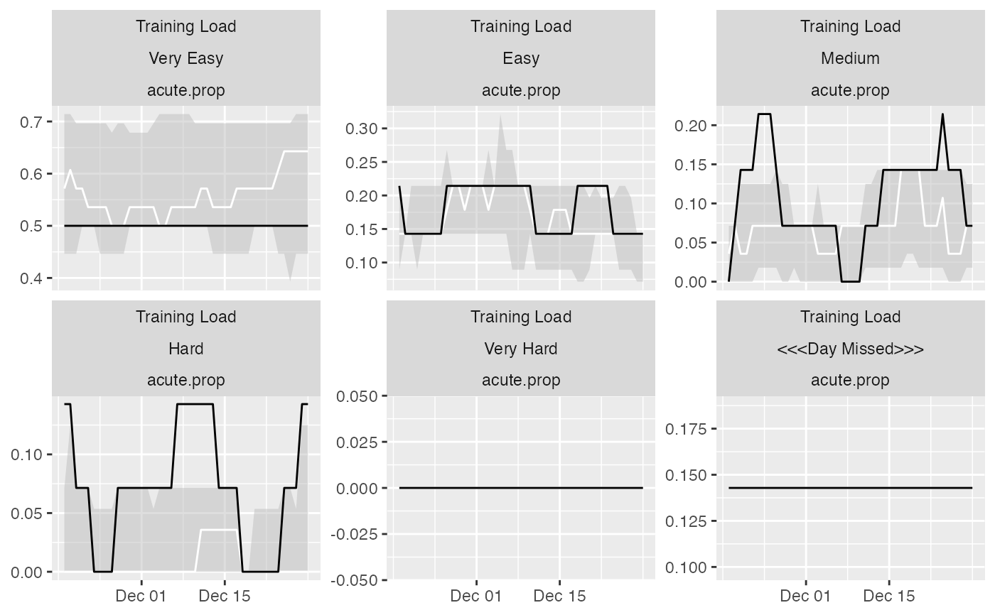
# Plots
plot(
prepared_data,
type = "line",
# To filter out athletes
athlete_name = "Ann Whitaker",
# To filter out variables
variable_name = "Training Load",
# To filter out estimators
estimator_name = "acute.prop",
group_lower_name = "group.lower",
group_central_name = "group.median",
group_upper_name = "group.upper",
trellis = TRUE
)
# Nominal data
# Create nominal variable
monitoring$Value_nominal <- cut(
monitoring$Value,
breaks = 5,
labels = c("Very Easy", "Easy", "Medium", "Hard", "Very Hard"),
include.lowest = TRUE
)
# Run the athlete monitoring data preparation
prepared_data <- prepare(
data = monitoring,
athlete = "Full Name",
date = "Date",
variable = "Variable",
value = "Value_nominal",
acute = 7,
chronic = 42,
# How should be missing entry treated?
NA_session = "<<<Session Missed>>>",
# How should missing days (i.e. no entries) be treated?
NA_day = "<<<Day Missed>>>",
# How should be multiple day entries summarised?
# This is different with levels, for example
# when there are two sessions, one is Low and one Hard
# if you use mean, then Low and Hard will be 0.5, with sum
# both will be 0.5, in which case the level probabilities will be
# summed to 1
day_aggregate = function(x) {
mean(x, na.rm = TRUE)
},
# Rolling estimators for Acute and Chronic windows
rolling_estimators = function(x) {
c(
"prop" = mean(x, na.rm = TRUE)
)
},
# Additional estimator post-rolling
posthoc_estimators = function(data) {
data$ACD <- data$acute.prop - data$chronic.prop
data$ACR <- data$acute.prop / data$chronic.prop
# Make sure to return the data
return(data)
},
# Group summary estimators
group_summary_estimators = function(x) {
c(
"median" = median(x, na.rm = TRUE),
"lower" = quantile(x, 0.25, na.rm = TRUE)[[1]],
"upper" = quantile(x, 0.75, na.rm = TRUE)[[1]]
)
}
)
#> Using nominal approach: column 'value' in the 'data' provided is not numeric. It will be treated as nominal and each level will be analyzed as separate variable using rolling counts approach.
#> Preparing data...
#> Rolling...
#> Group summaries...
#> Missing data summaries...
#> Done!
prepared_data
#> Athlete monitoring nominal data with the following characteristics:
#>
#> 10 athletes:
#> Alan McDonald, Ann Whitaker, Eve Black, Frank West, John Doe, Michael Peterson, Mike Smith, Peter Jackson, Stuart Rogan, Susan Kane
#>
#> 363 days:
#> From 18263 to 18625
#>
#> 34260 total entries
#>
#> 0 missing entries
#> 510 missing days
#> 0 extended days
#>
#> 1 variables:
#> Training Load
#>
#> 6 levels:
#> <<<Day Missed>>>, Easy, Hard, Medium, Very Easy, Very Hard
#>
#> 5 estimators:
#> variable.value, acute.prop, chronic.prop, ACD, ACR
summary(prepared_data)
#> # A tibble: 60 × 11
#> athlete variable level `Total entries` `Day entries` `Missing entries`
#> <chr> <chr> <chr> <int> <int> <dbl>
#> 1 Alan McDonald Training… <<<D… 571 363 0
#> 2 Alan McDonald Training… Easy 571 363 0
#> 3 Alan McDonald Training… Hard 571 363 0
#> 4 Alan McDonald Training… Medi… 571 363 0
#> 5 Alan McDonald Training… Very… 571 363 0
#> 6 Alan McDonald Training… Very… 571 363 0
#> 7 Ann Whitaker Training… <<<D… 571 363 0
#> 8 Ann Whitaker Training… Easy 571 363 0
#> 9 Ann Whitaker Training… Hard 571 363 0
#> 10 Ann Whitaker Training… Medi… 571 363 0
#> # ℹ 50 more rows
#> # ℹ 5 more variables: `Missing days` <int>, `Extended days` <int>,
#> # `Start date` <dbl>, `Stop date` <dbl>, Proportion <dbl>
# Plots
plot(
prepared_data,
type = "line",
# To filter out athletes
athlete_name = "Ann Whitaker",
# To filter out variables
variable_name = "Training Load",
# To filter out estimators
estimator_name = "acute.prop",
group_lower_name = "group.lower",
group_central_name = "group.median",
group_upper_name = "group.upper",
trellis = TRUE
)