athletemonitoring

Athlete monitoring data often comes in a form of time series or panel data. The goal of athletemonitoring package is to help in preparing these types of datasets using contemporary best practices which involve dealing with missing values, aggregating data on a day-level, creating rolling averages and finally providing visualizations.

Installation

You can install the released version of athletemonitoring from CRAN when it is available with:

install.packages("athletemonitoring")

And the development version from GitHub with:

# install.packages("devtools")
devtools::install_github("mladenjovanovic/athletemonitoring")

Example

athletemonitoring package is very simple package consisting of only the prepare() function and S3 methods for printing, summarizing, and plotting. Plotting features in athletemonitoring package are very powerful and flexible and allow you to create table, bar, line, and calendar heatmap plots.

require(athletemonitoring)
#> Loading required package: athletemonitoring

# Load monitoring data set
data("monitoring")

# Filter out only 'Training Load'
monitoring <- monitoring[monitoring$Variable == "Training Load", ]

# Convert column to date format (or use numeric)
monitoring$Date <- as.Date(monitoring$Date, "%Y-%m-%d")

# Run the athlete monitoring data preparation
prepared_data <- prepare(
  data = monitoring,
  athlete = "Full Name",
  date = "Date",
  variable = "Variable",
  value = "Value",
  acute = 7,
  chronic = 42,

  # How should be missing entry treated?
  # What do we assume? Zero load? Let's keep NA
  NA_session = NA,

  # How should missing days (i.e. no entries) be treated?
  # Here we assume no training, hence zero
  NA_day = 0,

  # How should be multiple day entries summarised?
  # With "load", it is a "sum", with other metrics that
  # do not aggregate, it can me "mean"
  day_aggregate = function(x) {
    sum(x, na.rm = TRUE)
  },

  # Rolling estimators for Acute and Chronic windows
  rolling_estimators = function(x) {
    c(
      "mean" = mean(x, na.rm = TRUE),
      "sd" = sd(x, na.rm = TRUE),
      "cv" = sd(x, na.rm = TRUE) / mean(x, na.rm = TRUE)
    )
  },

  # Additional estimator post-rolling
  posthoc_estimators = function(data) {
    data$ACD <- data$acute.mean - data$chronic.mean
    data$ACR <- data$acute.mean / data$chronic.mean
    data$ES <- data$ACD / data$chronic.sd

    # Make sure to return the data
    return(data)
  },

  # Group summary estimators
  group_summary_estimators = function(x) {
    c(
      "median" = median(x, na.rm = TRUE),
      "lower" = quantile(x, 0.25, na.rm = TRUE)[[1]],
      "upper" = quantile(x, 0.75, na.rm = TRUE)[[1]]
    )
  }
)
#> Preparing data...
#> Rolling...
#> Group summaries...
#> Missing data summaries...
#> Done!

# Get summary
prepared_data
#> Athlete monitoring numeric data with the following characteristics:
#> 
#> 10 athletes:
#> Alan McDonald, Ann Whitaker, Eve Black, Frank West, John Doe, Michael Peterson, Mike Smith, Peter Jackson, Stuart Rogan, Susan Kane 
#> 
#> 363 days:
#> From 18263 to 18625 
#> 
#> 5200 total entries
#> 
#> 0 missing entries
#> 510 missing days
#> 0 extended days
#> 
#> 1 variables:
#> Training Load 
#> 
#> 10 estimators:
#> variable.value, acute.mean, acute.sd, acute.cv, chronic.mean, chronic.sd, chronic.cv, ACD, ACR, ES

summary(prepared_data)
#> # A tibble: 10 × 16
#>    athlete          variable     `Total entries` `Day entries` `Missing entries`
#>    <chr>            <chr>                  <dbl>         <int>             <dbl>
#>  1 Alan McDonald    Training Lo…             520           363                 0
#>  2 Ann Whitaker     Training Lo…             520           363                 0
#>  3 Eve Black        Training Lo…             520           363                 0
#>  4 Frank West       Training Lo…             520           363                 0
#>  5 John Doe         Training Lo…             520           363                 0
#>  6 Michael Peterson Training Lo…             520           363                 0
#>  7 Mike Smith       Training Lo…             520           363                 0
#>  8 Peter Jackson    Training Lo…             520           363                 0
#>  9 Stuart Rogan     Training Lo…             520           363                 0
#> 10 Susan Kane       Training Lo…             520           363                 0
#> # ℹ 11 more variables: `Missing days` <int>, `Extended days` <int>,
#> #   `Start date` <dbl>, `Stop date` <dbl>, Mean <dbl>, SD <dbl>, Min <dbl>,
#> #   Max <dbl>, Median <dbl>, IQR <dbl>, MAD <dbl>


## Plots

# Table plot
# Produces formattable output with sparklines
# This will not work in the readme file, so just copy paste to your console
# plot(
#  prepared_data,
#  type = "table",
#
#  # Use to filter out estimators
#  estimator_name = c("acute.mean", "chronic.mean", "ES", "chronic.sd", "chronic.cv"),
#
#  # Use to filter out athlete
#  # athlete_name = NULL,
#
#  # Use to filter out variables
#  #variable_name = NULL,
#
#  # Show last entries
#  last_n = 42,
#
#  # Round numbers
#  digits = 2
# )

# Bar plot
# To plot group average
plot(
  prepared_data,
  type = "bar"
)
#> Plotting average across athletes. Please select athlete or use `trellis=TRUE`
#> Warning: Removed 42 rows containing missing values or values outside the scale range
#> (`geom_line()`).
#> Removed 42 rows containing missing values or values outside the scale range
#> (`geom_line()`).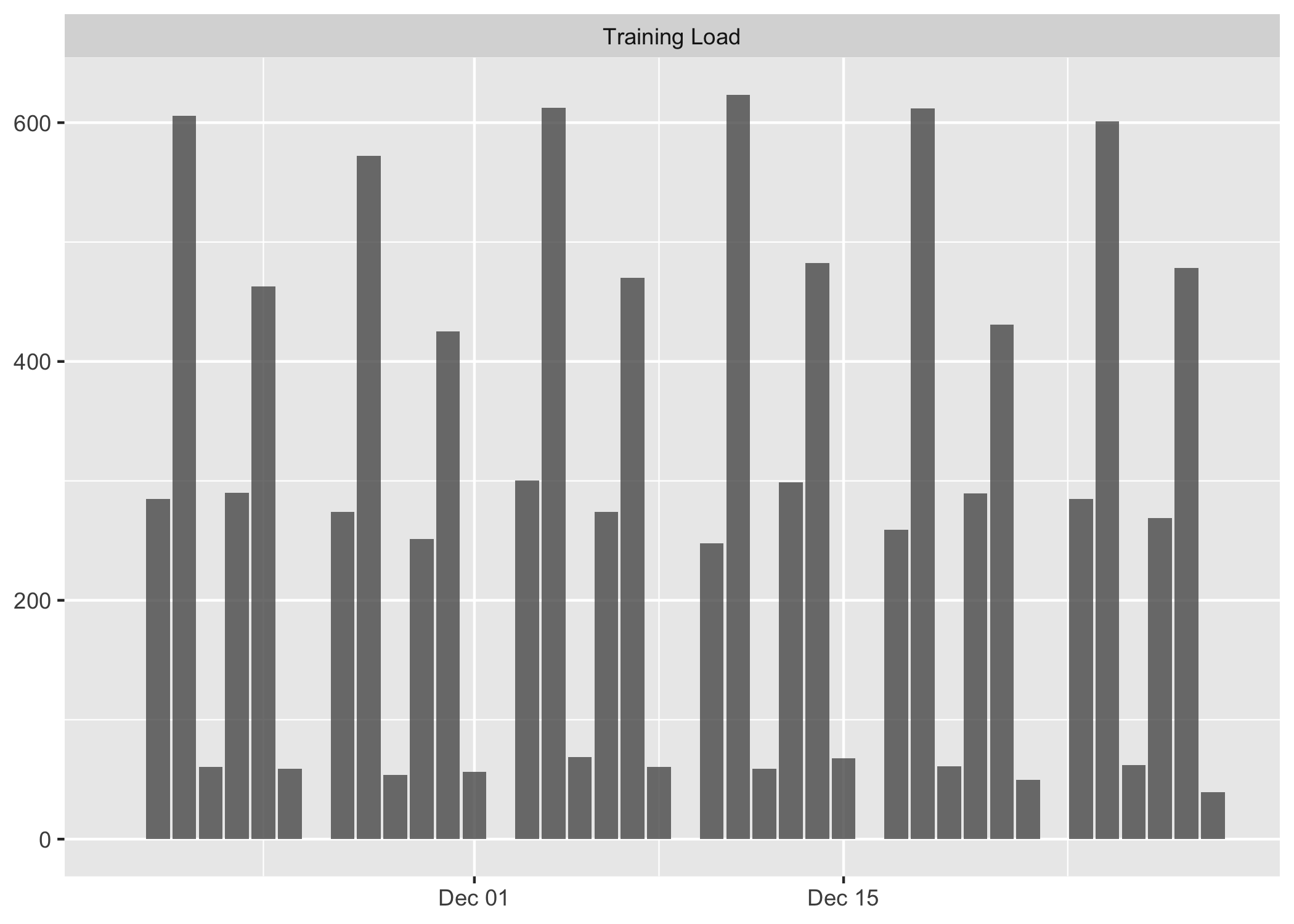

# To plot per athlete, use trellis argument
plot(
  prepared_data,
  type = "bar",
  trellis = TRUE
)
#> Warning: Removed 420 rows containing missing values or values outside the scale range
#> (`geom_line()`).
#> Warning: Removed 420 rows containing missing values or values outside the scale range
#> (`geom_line()`).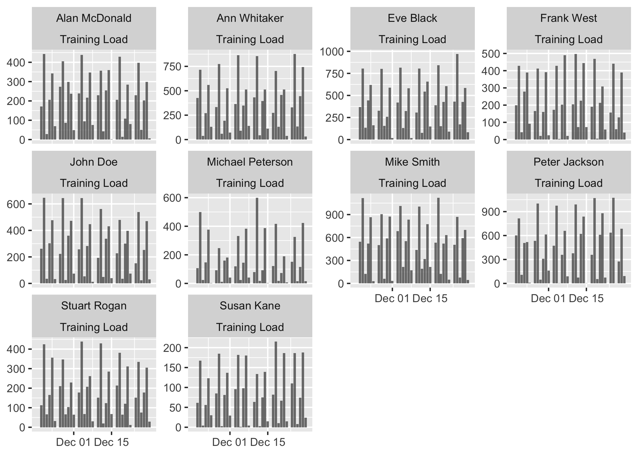

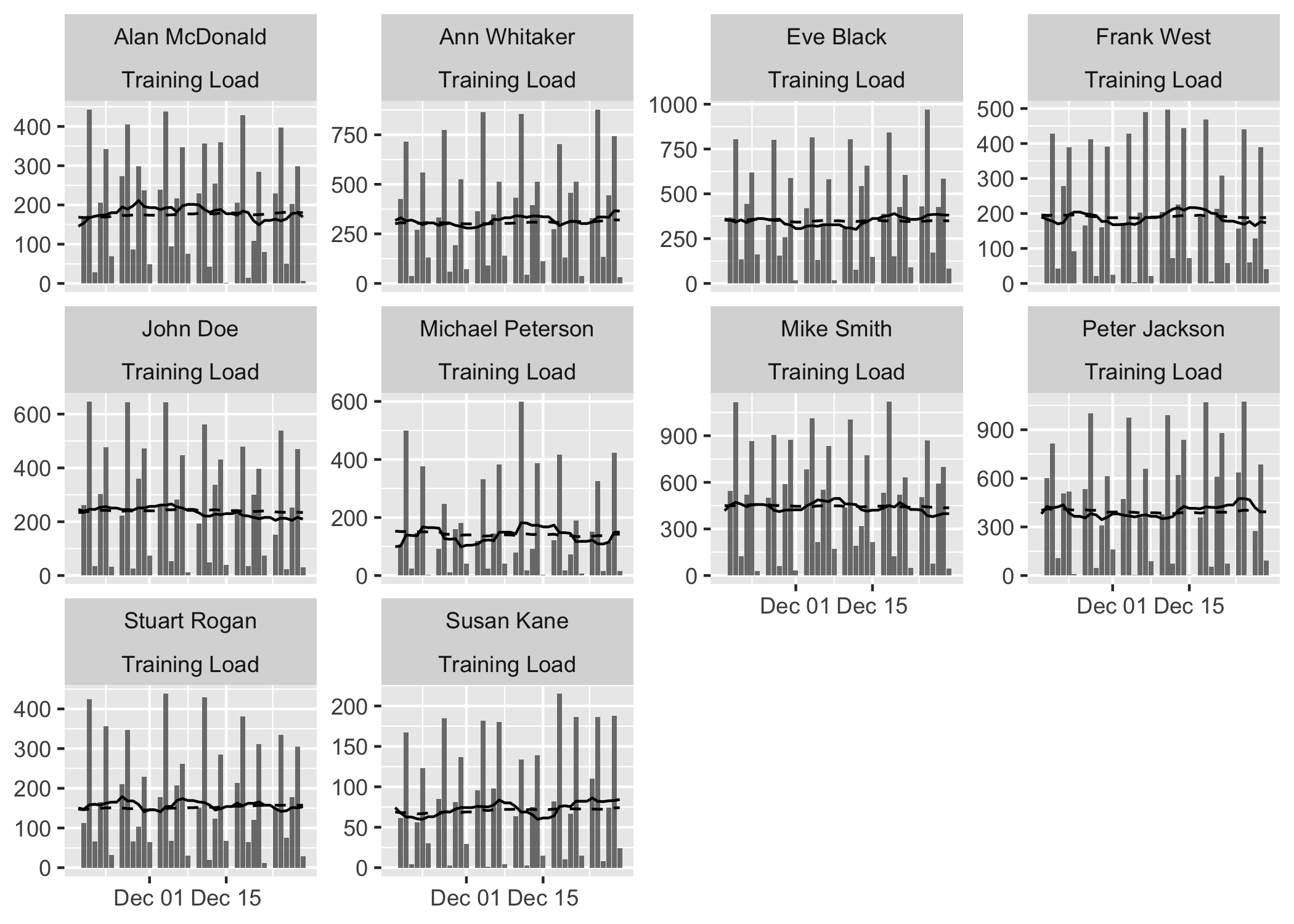
# To filter out athletem variable and add Acute and Chronic lines to the group average:
plot(
  prepared_data,
  type = "bar",

  # To filter out athletes
  # athlete_name = NULL,

  # To filter out variable
  # variable_name = NULL,

  # Add acute mean
  acute_name = "acute.mean",

  # Add chronic mean
  chronic_name = "chronic.mean",

  # Plot last n entries/days
  last_n = 42
)
#> Plotting average across athletes. Please select athlete or use `trellis=TRUE`

# If you want to plot for each athlete, use trellis=TRUE
plot(
  prepared_data,
  type = "bar",
  acute_name = "acute.mean",
  chronic_name = "chronic.mean",
  last_n = 42,
  trellis = TRUE
)

# Line plots
# These plots represent summary of the rollins estimators
plot(
  prepared_data,
  type = "line",

  # To filter out athletes
  # athlete_name = NULL,

  # To filter out variables
  # variable_name = NULL,

  # To filter out estimators
  # estimator_name = NULL,

  # Tell graph where the lower group estimator is
  # which is in this case 25%th percentile of the group
  group_lower_name = "group.lower",

  # The name of the centrality estimator of the group
  group_central_name = "group.median",

  # Tell graph where the upper group estimator is
  # which is in this case 75%th percentile of the group
  group_upper_name = "group.upper",

  # Use trellis if you do not plot for a single individual
  trellis = TRUE
)

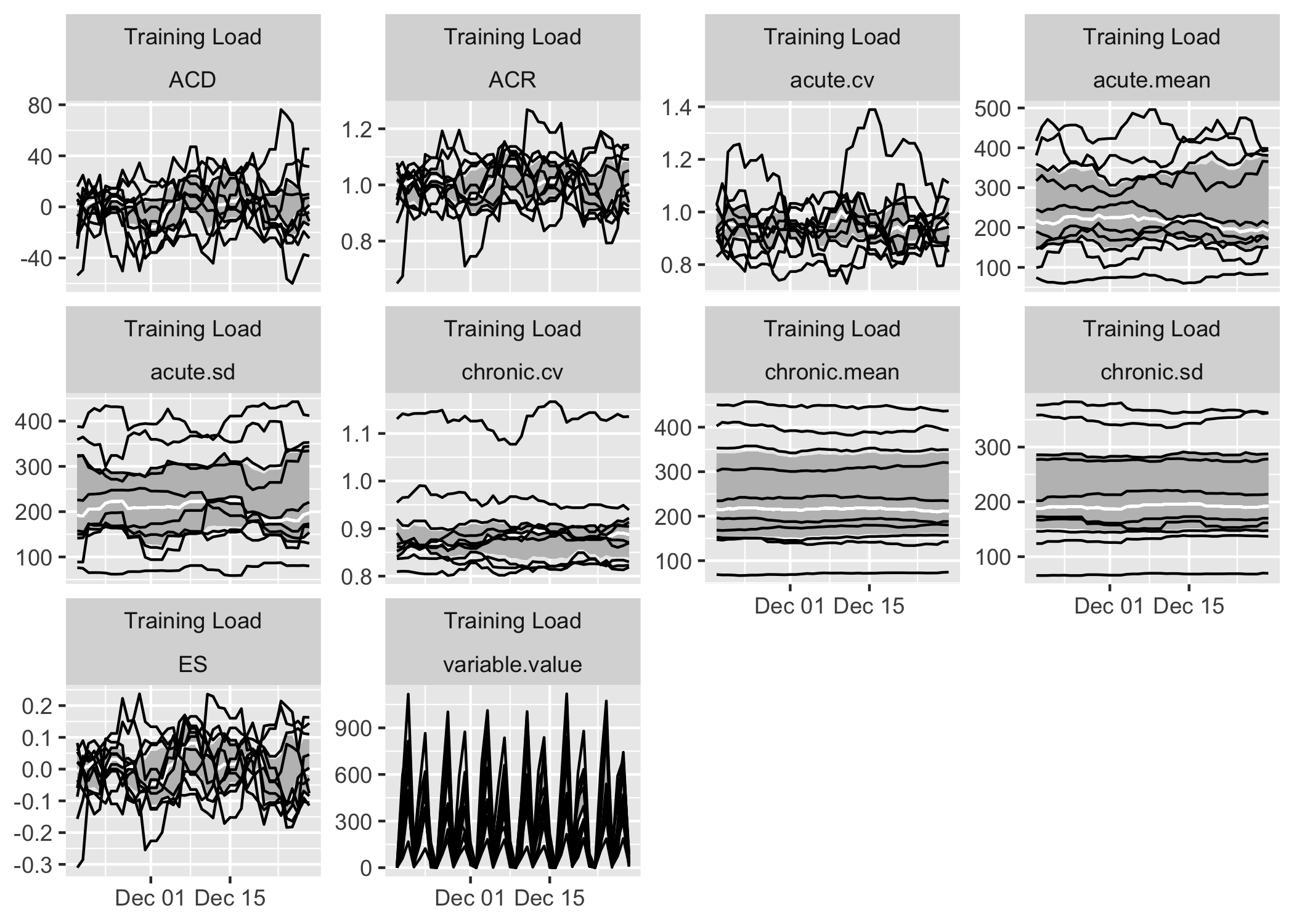
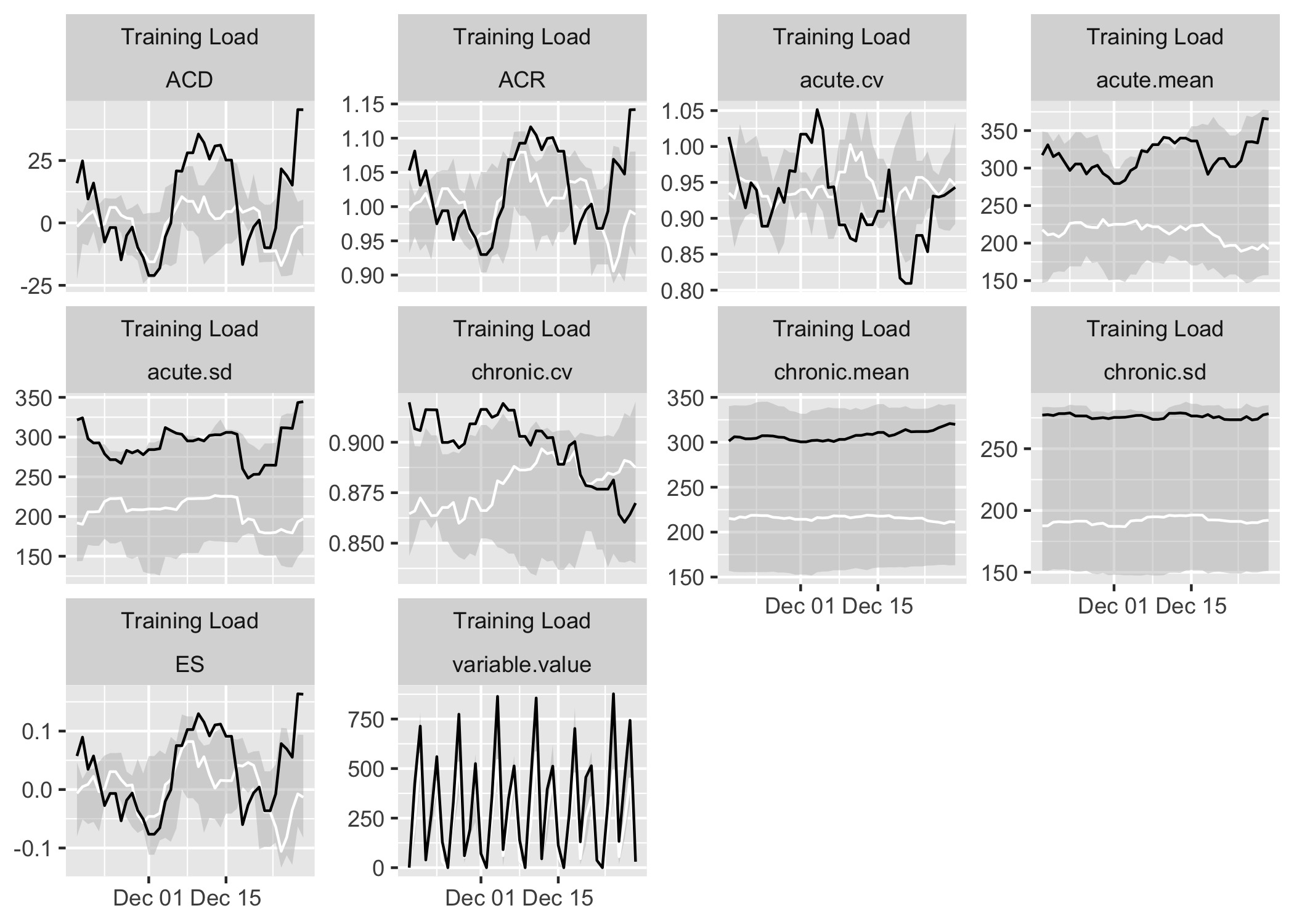
# Previous chart looks messy because it plot all athletes
# To avoid that, filter out only one athlete
plot(
  prepared_data,
  type = "line",

  # To filter out athletes
  athlete_name = "Ann Whitaker",
  group_lower_name = "group.lower",
  group_central_name = "group.median",
  group_upper_name = "group.upper",
  trellis = TRUE
)

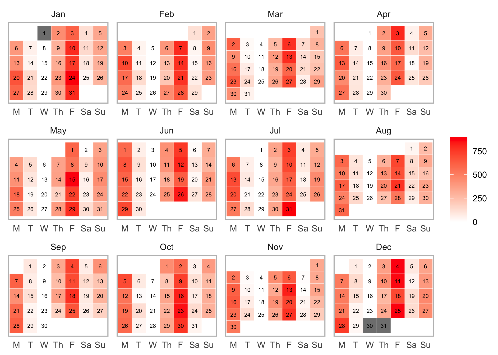
# Calendar heatmap plot
plot(
  prepared_data,
  type = "calendar",
  
  # To filter out athletes
  athlete_name = "Ann Whitaker",
  
  # To filter out variables
  variable_name = "Training Load",
  
  # To print estimator
  estimator_name = "variable.value", # Or use "entries"
  
  # To filter out last days
  last_n = 365,
  
  # To setup colors
  low_color = "white",
  high_color = "red",
  na_color = "grey50",
  
  # Should the whole year be plotted?
  # Otherwise full months are plotted
  full_year = TRUE,
  
  # Should year label be plotted? 
  # in the case of multiple years involved
  # it is always plotted
  year_label = FALSE,
  
  # Short weekdays?
  short_weekday = TRUE,
  
  # Label size
  label_size = 2,
  
  # Aggregation function in the case multiple athletes/variables/levels are used
  aggregate_func = mean
)

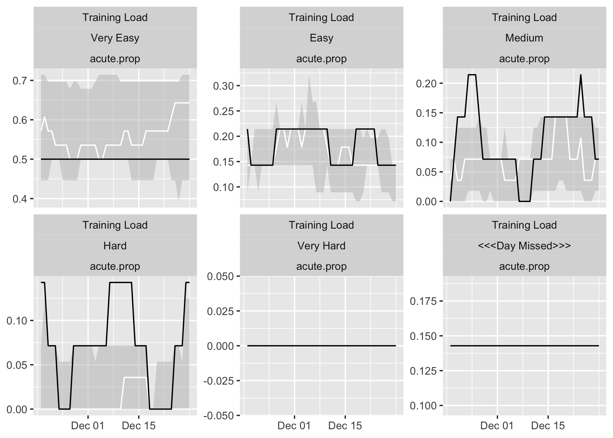
Example for nominal scale

Sometimes the data comes in nominal scale (e.g., Hard, Medium, Easy). Analysis of this type of data involves analysis of each levels independently, which results in rolling counts or rolling proportions.

# Create nominal variable
monitoring$Value_nominal <- cut(
  monitoring$Value,
  breaks = 5,
  labels = c("Very Easy", "Easy", "Medium", "Hard", "Very Hard"),
  include.lowest = TRUE
)


# Create a missing value
monitoring$Value_nominal[1] <- NA

# Run the athlete monitoring data preparation
prepared_data <- prepare(
  data = monitoring,
  athlete = "Full Name",
  date = "Date",
  variable = "Variable",
  value = "Value_nominal",
  acute = 7,
  chronic = 42,

  # How should be missing entry treated?
  NA_session = "<<<Session Missed>>>",

  # How should missing days (i.e. no entries) be treated?
  NA_day = "<<<Day Missed>>>",

  # How should be multiple day entries summarised?
  # With "load", it is a "sum", with other metrics that
  # do not aggregate, it can me "mean"
  day_aggregate = function(x) {
    sum(x, na.rm = TRUE)
  },

  # Rolling estimators for Acute and Chronic windows
  rolling_estimators = function(x) {
    c(
      "mean" = mean(x, na.rm = TRUE),
      "sd" = sd(x, na.rm = TRUE),
      "cv" = sd(x, na.rm = TRUE) / mean(x, na.rm = TRUE)
    )
  },

  # Additional estimator post-rolling
  posthoc_estimators = function(data) {
    data$ACD <- data$acute.mean - data$chronic.mean
    data$ACR <- data$acute.mean / data$chronic.mean
    data$ES <- data$ACD / data$chronic.sd

    # Make sure to return the data
    return(data)
  },

  # Group summary estimators
  group_summary_estimators = function(x) {
    c(
      "median" = median(x, na.rm = TRUE),
      "lower" = quantile(x, 0.25, na.rm = TRUE)[[1]],
      "upper" = quantile(x, 0.75, na.rm = TRUE)[[1]]
    )
  }
)
#> Using nominal approach: column 'value' in the 'data' provided is not numeric. It will be treated as nominal and each level will be analyzed as separate variable using rolling counts approach.
#> Preparing data...
#> Rolling...
#> Group summaries...
#> Missing data summaries...
#> Done!

# Get summary
prepared_data
#> Athlete monitoring nominal data with the following characteristics:
#> 
#> 10 athletes:
#> Alan McDonald, Ann Whitaker, Eve Black, Frank West, John Doe, Michael Peterson, Mike Smith, Peter Jackson, Stuart Rogan, Susan Kane 
#> 
#> 363 days:
#> From 18263 to 18625 
#> 
#> 39970 total entries
#> 
#> 1 missing entries
#> 510 missing days
#> 0 extended days
#> 
#> 1 variables:
#> Training Load 
#> 
#> 7 levels:
#> <<<Day Missed>>>, <<<Session Missed>>>, Easy, Hard, Medium, Very Easy, Very Hard 
#> 
#> 10 estimators:
#> variable.value, acute.mean, acute.sd, acute.cv, chronic.mean, chronic.sd, chronic.cv, ACD, ACR, ES

# Nominal data
# Create nominal variable
monitoring$Value_nominal <- cut(
  monitoring$Value,
  breaks = 5,
  labels = c("Very Easy", "Easy", "Medium", "Hard", "Very Hard"),
  include.lowest = TRUE
)

# Run the athlete monitoring data preparation
prepared_data <- prepare(
  data = monitoring,
  athlete = "Full Name",
  date = "Date",
  variable = "Variable",
  value = "Value_nominal",
  acute = 7,
  chronic = 42,

  # How should be missing entry treated?
  NA_session = "<<<Session Missed>>>",

  # How should missing days (i.e. no entries) be treated?
  NA_day = "<<<Day Missed>>>",

  # How should be multiple day entries summarised?
  # This is different with levels, for example
  # when there are two sessions, one is Low and one Hard
  # if you use mean, then Low and Hard will be 0.5, with sum
  # both will be 0.5, in which case the level probabilities will be
  # summed to 1
  day_aggregate = function(x) {
    mean(x, na.rm = TRUE)
  },

  # Rolling estimators for Acute and Chronic windows
  rolling_estimators = function(x) {
    c(
      "prop" = mean(x, na.rm = TRUE)
    )
  },

  # Additional estimator post-rolling
  posthoc_estimators = function(data) {
    data$ACD <- data$acute.prop - data$chronic.prop
    data$ACR <- data$acute.prop / data$chronic.prop

    # Make sure to return the data
    return(data)
  },

  # Group summary estimators
  group_summary_estimators = function(x) {
    c(
      "median" = median(x, na.rm = TRUE),
      "lower" = quantile(x, 0.25, na.rm = TRUE)[[1]],
      "upper" = quantile(x, 0.75, na.rm = TRUE)[[1]]
    )
  }
)
#> Using nominal approach: column 'value' in the 'data' provided is not numeric. It will be treated as nominal and each level will be analyzed as separate variable using rolling counts approach.
#> Preparing data...
#> Rolling...
#> Group summaries...
#> Missing data summaries...
#> Done!

prepared_data
#> Athlete monitoring nominal data with the following characteristics:
#> 
#> 10 athletes:
#> Alan McDonald, Ann Whitaker, Eve Black, Frank West, John Doe, Michael Peterson, Mike Smith, Peter Jackson, Stuart Rogan, Susan Kane 
#> 
#> 363 days:
#> From 18263 to 18625 
#> 
#> 34260 total entries
#> 
#> 0 missing entries
#> 510 missing days
#> 0 extended days
#> 
#> 1 variables:
#> Training Load 
#> 
#> 6 levels:
#> <<<Day Missed>>>, Easy, Hard, Medium, Very Easy, Very Hard 
#> 
#> 5 estimators:
#> variable.value, acute.prop, chronic.prop, ACD, ACR

summary(prepared_data)
#> # A tibble: 60 × 11
#>    athlete       variable  level `Total entries` `Day entries` `Missing entries`
#>    <chr>         <chr>     <chr>           <int>         <int>             <dbl>
#>  1 Alan McDonald Training… <<<D…             571           363                 0
#>  2 Alan McDonald Training… Easy              571           363                 0
#>  3 Alan McDonald Training… Hard              571           363                 0
#>  4 Alan McDonald Training… Medi…             571           363                 0
#>  5 Alan McDonald Training… Very…             571           363                 0
#>  6 Alan McDonald Training… Very…             571           363                 0
#>  7 Ann Whitaker  Training… <<<D…             571           363                 0
#>  8 Ann Whitaker  Training… Easy              571           363                 0
#>  9 Ann Whitaker  Training… Hard              571           363                 0
#> 10 Ann Whitaker  Training… Medi…             571           363                 0
#> # ℹ 50 more rows
#> # ℹ 5 more variables: `Missing days` <int>, `Extended days` <int>,
#> #   `Start date` <dbl>, `Stop date` <dbl>, Proportion <dbl>

# Plots
plot(
  prepared_data,
  type = "line",

  # To filter out athletes
  athlete_name = "Ann Whitaker",

  # To filter out variables
  variable_name = "Training Load",

  # To filter out estimators
  estimator_name = "acute.prop",
  group_lower_name = "group.lower",
  group_central_name = "group.median",
  group_upper_name = "group.upper",
  trellis = TRUE
)

Further information

To find out more, please check the Athlete Monitoring Course, which covers a lot of ground and the utilization of the athletemonitoring package in depth.